
Space nerds have an old saying that ‘LEO is half way to the moon…‘ and Arduino hobbyists tend to feel the same way about getting sensor readings displayed on a live IoT dashboard. But that ignores the real work it takes to generate data that’s actually useable. To paraphrase Heinlein: ‘Calibration is half way to anywhere…’ Now that our 2-Part logger is both easy for students to build and robust enough for field use, we can focus on developing sensor calibration methods that are achievable by teachers and researchers in low-resource settings.
Light sensors seem straight forward, with numerous how-to guides at Hackaday, Adafruit, Sparkfun, etc. In reality, light sensors are some of the trickiest ones to actually deploy – which is why so few low-end climate stations include them. This post describes a method for calibrating a Bh1750 lux sensor to estimate Photosynthetically Active Radiation (PAR). Not everyone can afford a LI-COR 190 or Apogee SQ quantum sensor to use as a benchmark, so here we will use a clear-sky model calculation for the cross-calibration despite the dynamic filtering effects of the atmosphere on natural sunlight. Using a diffuser to restore cosign behavior means we can’t calculate PPFD directly from Lux without some y=mx+b coefficients.
Jump links to the sections of this post:
- Issue #1: Spectral Distribution
- Issue #2: Sensitivity Bands
- Issue #3: Sensor Range
- Issue #4: Angular Response
- Issue #5: Temporal Resolution
- The Radiation Shield
- A Leveling Mount / Mechanism
- The Apogee Clear Sky Calculator
- Our Deployment Location
- The Calibration
- Discussion
Light Sensor Issue #1: Changing Spectral Distribution

Peak solar irradiance received on any given day varies by latitude and season, as does the overall pattern. Light emitted from the sun has a stable distribution of frequencies, however the spectrum at the earth’s surface varies across the day, with more short wavelengths (blue) around mid day and enriched in longer wavelengths (red) at sunrise & sunset when the rays travel further through the atmosphere. We will avoid this source of error by calibrating with data from the hours around solar noon as determined by the NOAA Solar Calculator. Even with high quality sensors, morning and evening data can be compromised by other factors like condensation which changes the refractive index of lenses and diffusers.
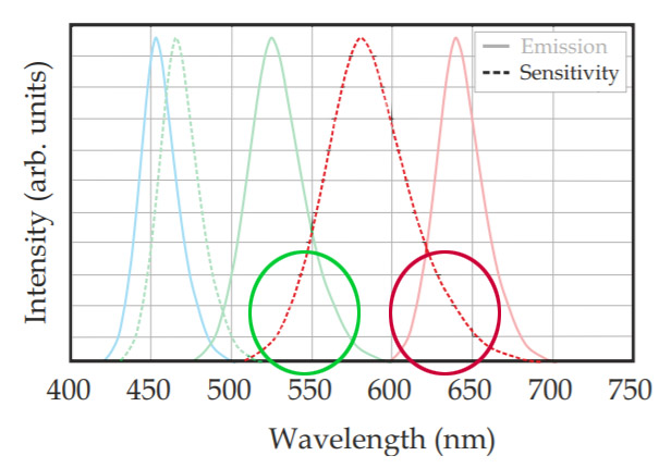
Light Sensor Issue #2: Sensitivity Bands

Lux sensors have a maximum sensitivity near 550nm, mimicking the response of photo-receptors in the human eye. Plants are similarly limited to frequencies that can be absorbed by the various chlorophylls. These two bands have a high degree of overlap so we can avoid the Badder UV/IR-Cut cut filters (420–685nm bandpass) or stack of Roscolux filters that would be needed with photodiodes that respond to a wider range of incoming radiation. The cross-calibration still requires the relative ratio of frequencies within the targeted region to remain stable, so a PAR conversion derived under full sunlight may not be valid under a canopy of tree leaves or for the discontinuous spectra of ‘blurple’ grow-lights.
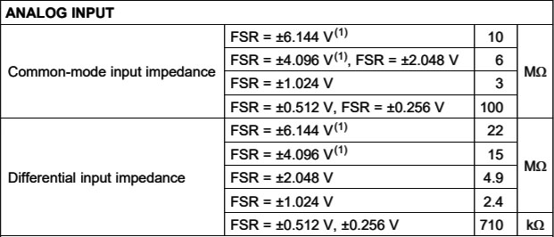
Light Sensor Issue #3: Dynamic Range

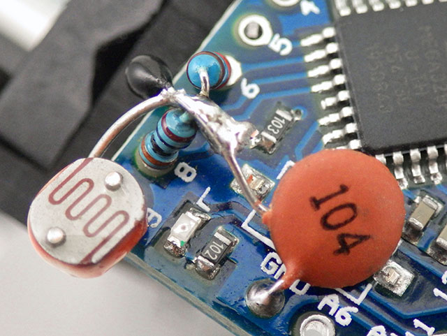
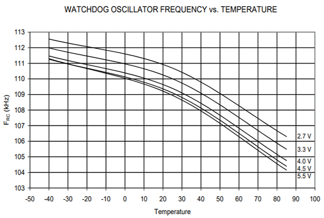
Full summer sunlight can exceed 120,000 Lux and there aren’t many sensors in the Arduino ecosystem that handle that entire range. The BH1750 can with registers set to it’s least sensitive configuration. Our logger code already does this because QUALITY_LOW & MTREG_LOW(31) integration take only 16-24 milliseconds, rather than the 120-180ms of power needed for high resolution readings. The data sheet implies that the sensor will flatline before 100,000 lux, but at its lowest sensitivity it delivers reasonable data above 120k, though linearity may be suspect as flux approaches sensor saturation. The sensor also has a maximum operating temperature of 85°C which can be exceeded if your housing suffers too much heat gain. Alternative sensors like the MAX44009, TSL2591 and SI1145 have a similar thermal limits. Like most light sensors, the Bh1750 increases its output readings by a few percent as the sensor warms.

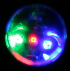
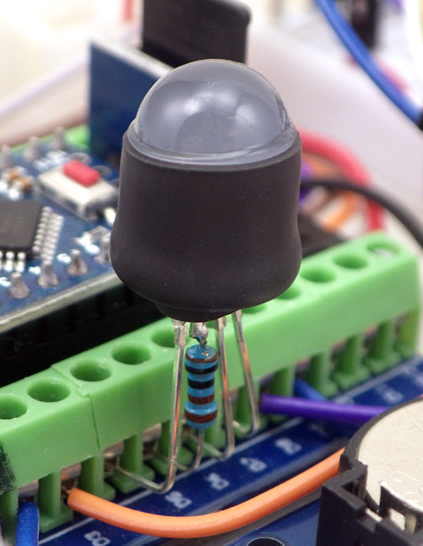
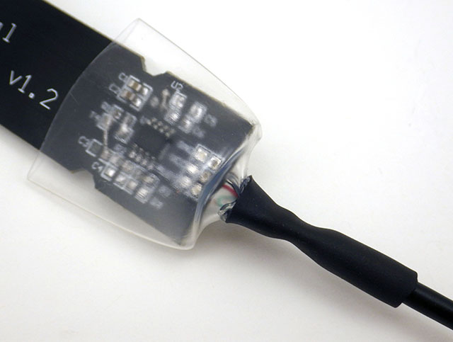
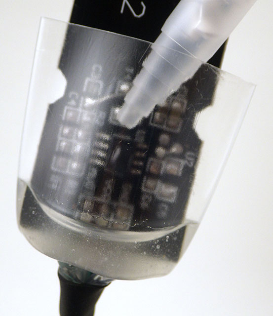
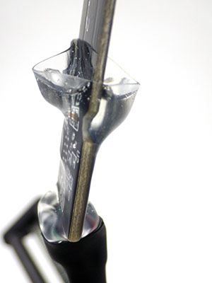
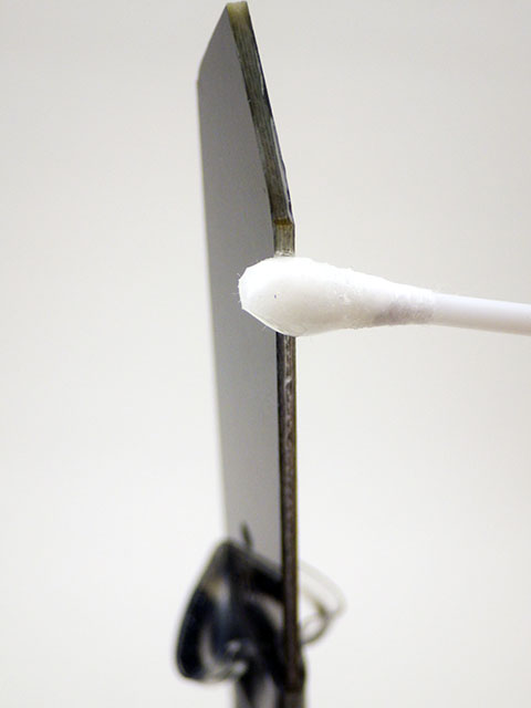
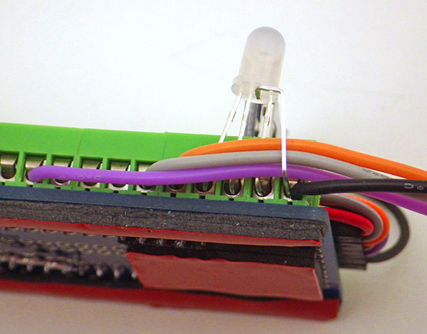
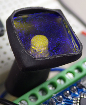
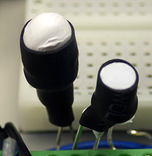
DIY builders often add diffusers made from translucent #7328 Acrylite or PTFE sheets to reduce sunlight intensity into a given sensors range. I tried printing domes with clear PETG and hand sanding them with fine grit to increase the diffusive power. While these did reduce light levels by more than 50%, my DIY diffuser didn’t quite match the smooth overall response seen with the diffusers that came with the round PCB modules. This may have been due to a slight misalignment between the sensor and the focal point of the low-poly dome I could make in Tinkercad. The white dome that comes with the red Bh1750 module reduced peak light levels in full sunlight from the 110k Lux reported by a ‘naked’ sensor to about 40k Lux. Each sensor varied somewhat in its response but I didn’t do any batch testing to quantify this as I was calibrating each sensor directly to the reference model. I initially tried clear JB weld as a sealant but this caused problems: sometimes contracting enough peel parts away from the PCB and yellowing significantly after a couple of weeks of full sun exposure. In later builds I used only a thin coating of silicone conformal, relying on an epoxy seal around the base of the diffuser to provide most of the waterproofing.
Light Sensor Issue #4: Angular Response

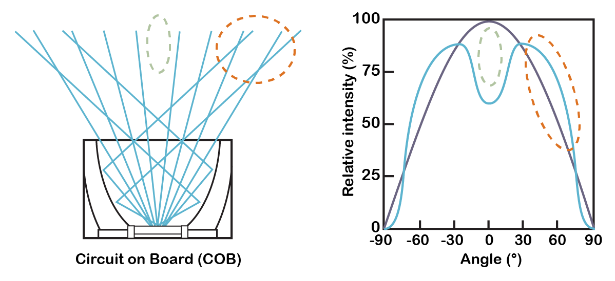
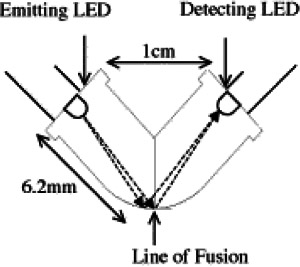
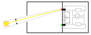
Lambert’s cosine law describes the relationship between the angle of incidence and the level of illuminance on a flat matte surface as being proportional to the cosine of the zenith angle (as the suns changes position throughout the day). At an incident angle of 60°, the number of photons hitting a sensor surface is half what it would be if the same light source was positioned directly above the sensor. This effect is mathematically predictable, but imperfections, diffraction, and surface reflection means that sensor response tends to diverge from ideal as the angle increases. So manufacturers surround their sensors with raised diffuser edges and recesses on the top surface which change light collection at low sun angles to restore a perfect cosign response. In general, diffusers make the compass orientation of the sensor less likely to interfere with calibration but leveling the sensor is still absolutely required.
Light Sensor Issue #5: Temporal Resolution
Unlike most environmental parameters, light levels can change instantaneously. Most commercial sensors aggregate 1 or 2 second readings into 5 to 15 minute averages. This makes it much easier to estimate energy output from solar panels, or calculate the Daily Light Integral for a crop because both of those use cases are more concerned with area under the curve rather than individual sensor readings. However, in our case of calibrating a sensor against an irradiance model, we must use instantaneous readings so we can exclude data from periods where the variability is high. Averaging would smooth over short term interference from clouds, birds, or overhead wires, potentially leading to bad data in the calibration. We read the BH1750 once per minute at its fastest/lowest resolution.
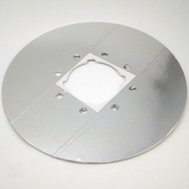
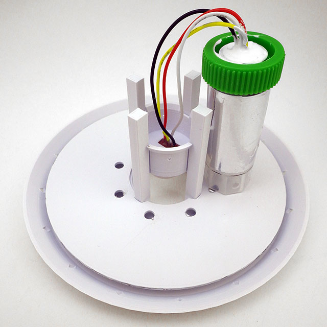
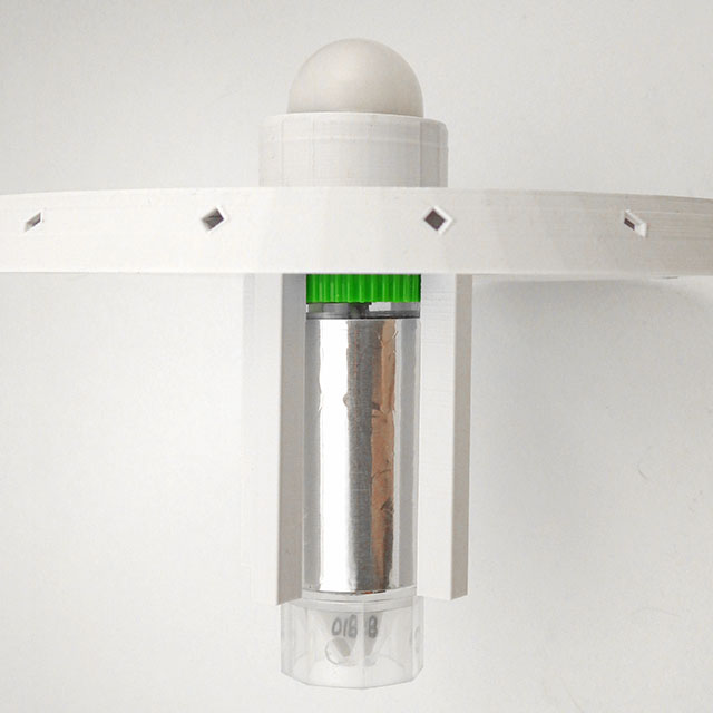
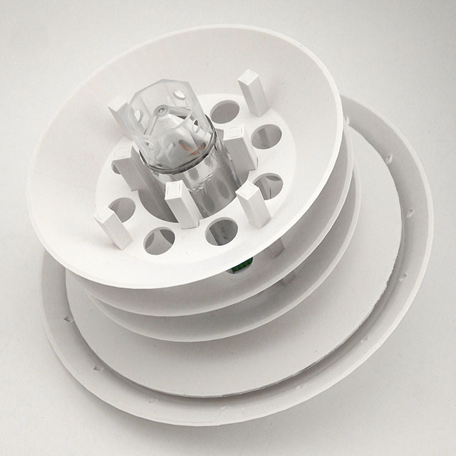
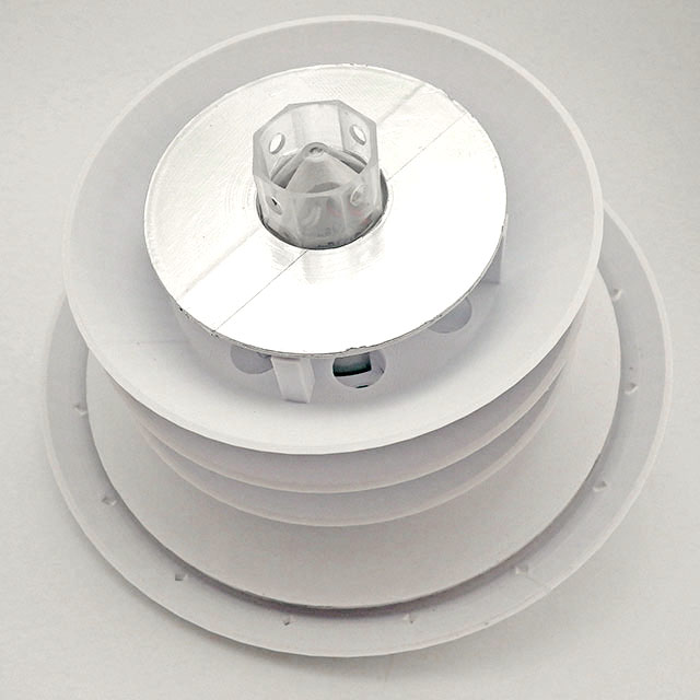
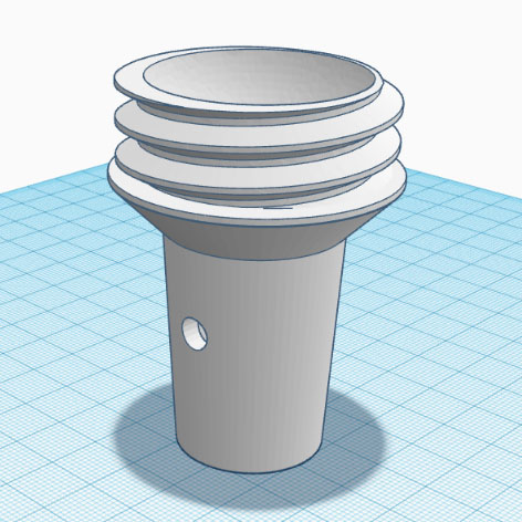
A Radiation Shield
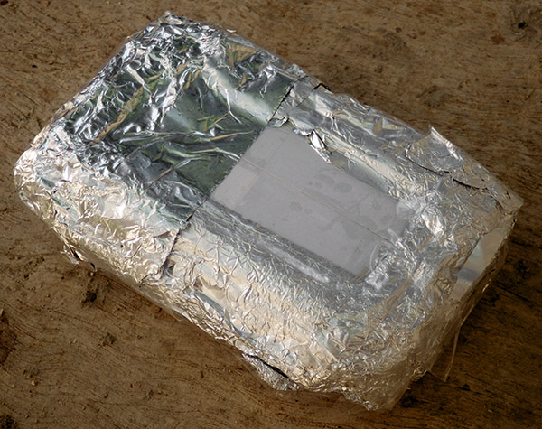
My original concept was to epoxy the light sensor directly onto the cap and slide separate radiation shields over the housing tube with a friction fit – but that approach suffered excessive heat gain. It took several design iterations to discover that plastics are often transparent to IR – so most of the 3D printed weather station shields you find in maker space won’t work very well. While PLA does block/reflect the visible spectrum, it then re-emits a portion of any absorbed energy as IR which passes right through – turning the central housing tube into a tiny greenhouse. You need to add layers of metal foil to reflect that IR and there must be an air gap between the materials or the heat still crosses by conduction. The process of moving those surfaces away from the logger also meant placing the sensor onto a small raised ‘stage’ that could pass through the upper shield. This allows easier replacement after the sensors expire, or the use of an entirely different sensor without changing the rest of the design. I still don’t know the operating life of these sensors at full sunlight exposure levels.

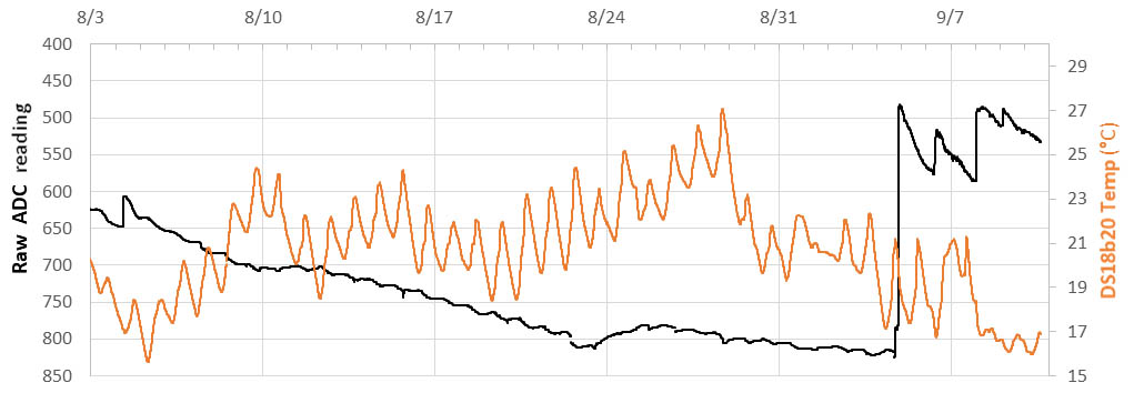
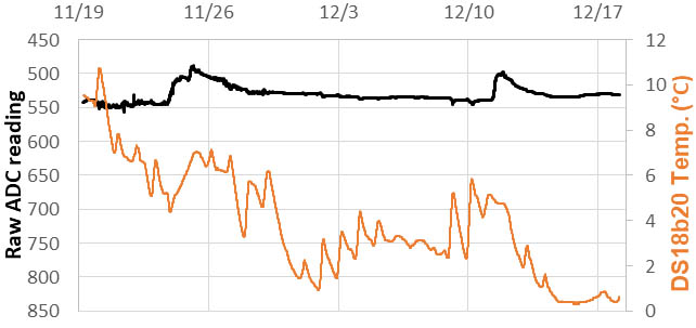
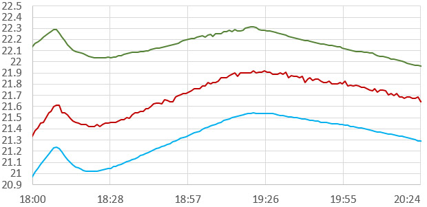
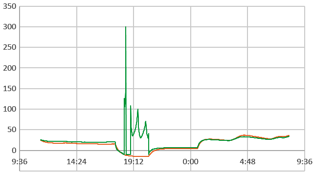
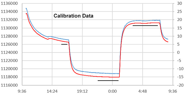
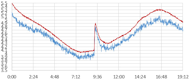
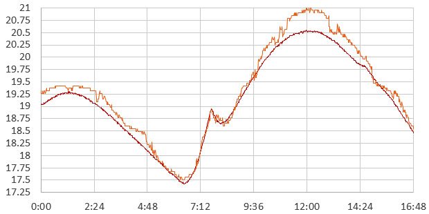
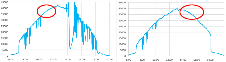
Here are temperature records of two side-by-side loggers with identical 3D-printed shields except that one has the three metal foil layers added and one does not:

Interestingly, the 3°C delta seen in my foil vs no foil tests matched the discrepancies identified by Terando et.al in their 2017 paper examining ad hoc Stevenson shields in ecological studies. Air gaps are required for IR reflecting layers to do their job, so most of the foil backed roofing shingles on the market are ineffective because of direct surface contact. Both aluminum and stainless steel foils are common, but aluminum has a lower emissivity than stainless steel, meaning it should reflect more and emit less IR. There are also radiant barrier coating sprays used in industrial settings. High-end weather stations use fan ventilation or helical shields, but those designs may be a bit too complicated for DIY. And even 3D prints from tough materials like PETG or ASA would benefit from coating with something like Krylon UV protectant to extend their lifespan. I’ve also been thinking about adding some infrared cooling paint on the top surface of our weather stations. The challenge with anything that emits in the atmospheres transparency window between wave lengths of 8 and 13 microns is that you get significant accumulation of debris on surfaces in as little as one month of actual deployment: especially in the spring/fall when the surfaces get covered with morning dew which then captures any windborne dust.
I’m still tweaking the shield design as more test data comes in, and hope to compare it to a fan aspirated model soon. Radiation shields are only needed if you want to capture accurate temperatures with the light readings on the same logger. The Bh1750 calibration alone could be done without shields, but mounting the sensor on some kind of flat surface makes it easier to add the required leveling bubble beside the sensor. The tradeoff for preventing solar heat gain is that shields introduce lag in the temperature response.
Pole Mount & Leveling Mechanism
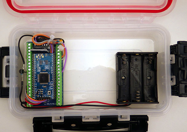
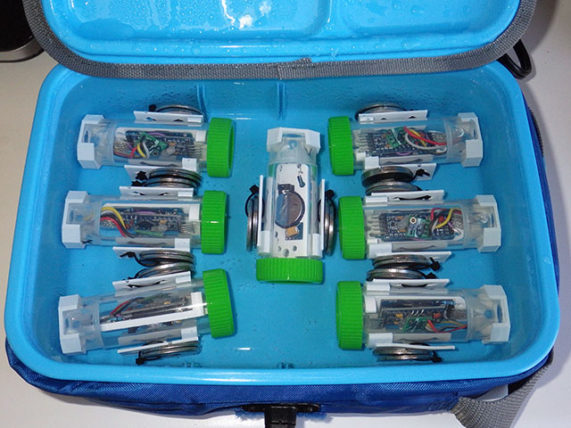
As this is the first of our ‘garden series’ that will be built around the 2-part logger, I created a complete mounting system from a combination of 3D printed parts and PVC pipes. This adjustable leveling mechanism was modified from the Open Source Universal Ball Joint posted on Thingiverse by Arthur ZOPFE.
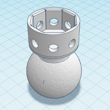
This ball & socket approach works well for leveling, but to make the adjustments easier (ie. with less compressive force) I will add an O-ring to the bottom cup for some friction and give.
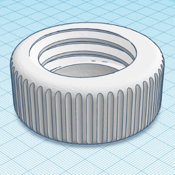
A length of standard 1/2 inch PVC pipe is used for the riser between the spike and the leveling mechanism. Ideal height for temperature sensors is approximately five feet above the ground, usually in a shaded location facing away from the sun.
The Apogee Clear Sky Calculator
The Apogee Clear Sky Calculator helps operators of their many light sensor products check if those need to be sent in for re-calibration. When used near solar noon on clear unpolluted days the accuracy is estimated to be ±4 %. We can cross-calibrate the readings from our humble Bh1750 to that model provided we use data from a cloudless day. I’m not sure what the temporal resolution of the ClearSky model is (?) The U.S. Climate Reference Network generally uses two-second readings averaged into five minute values so it is likely that the ClearkSky model has a similar resolution. This model has the best accuracy within one hour of solar noon but we will push that out a few hours so we have enough data for the regression.
We could have used the Bird Clear Sky Model from NREL, with validation against real world data from one of the local SURFRAD stations at NOAA. That data is for full-spectrum pyranometers measuring in W/m2, but you can estimate the PAR as photosynthetic photon flux density (PPFD) from total shortwave radiation using a conversion factor into µmol s-1 m-2. Many solar PV companies provide online calculators for power density that could also be used for this kind of DIY sensor calibration.
Our Deployment Location
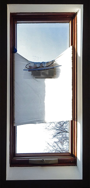
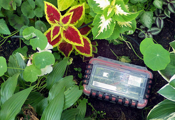
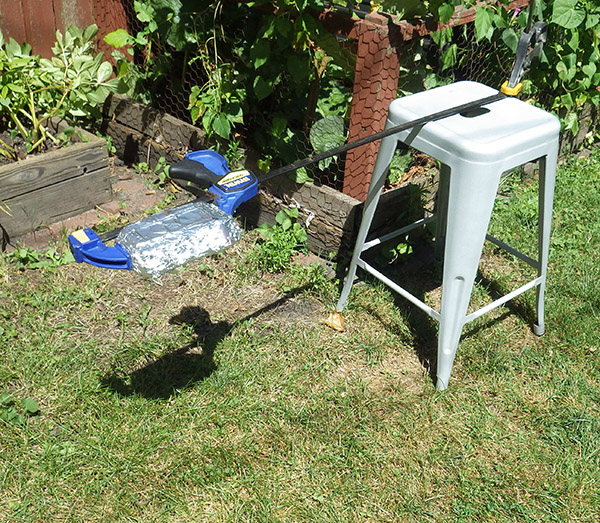
Most who live in urban areas are familiar with noise pollution, however it is also hard to find undisturbed light environments. My best option for those critical hours around solar noon was my neighbours backyard garden:
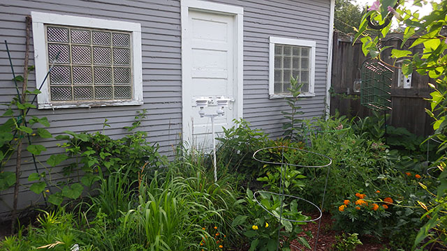
This location was relatively free of power lines and tree tops, but reflections from that white door caused a slight positive offset in the afternoon. Fences prevented the capture of morning and evening data which would have been interesting. But sunrise to sunset data is not required for our calibration.
The Calibration
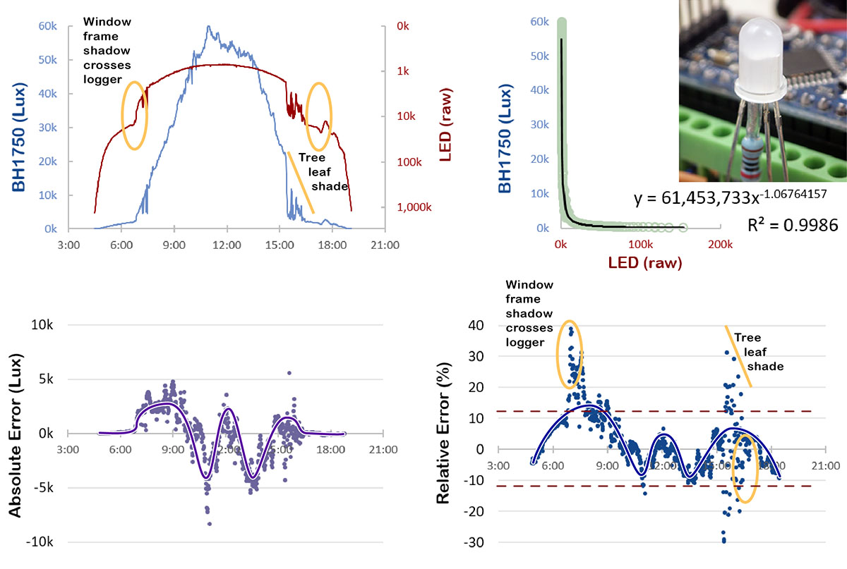
After several weeks of logger operation we finally managed to capture data from a beautiful cloud-free day:
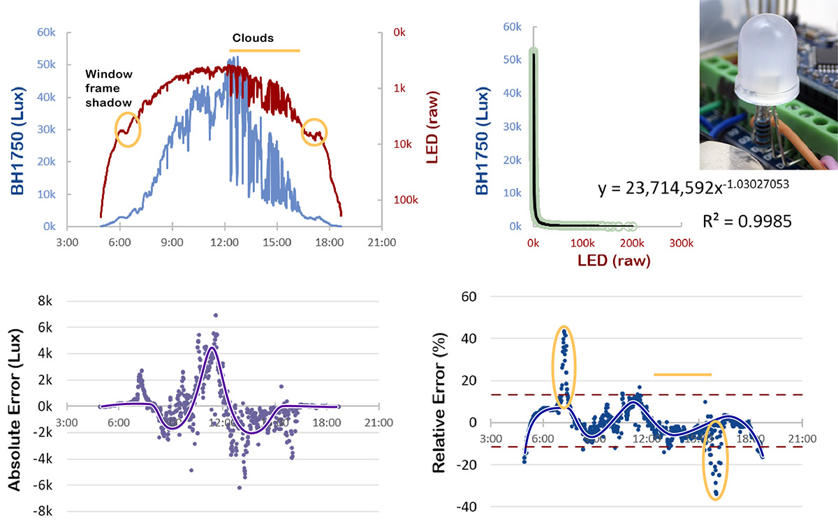
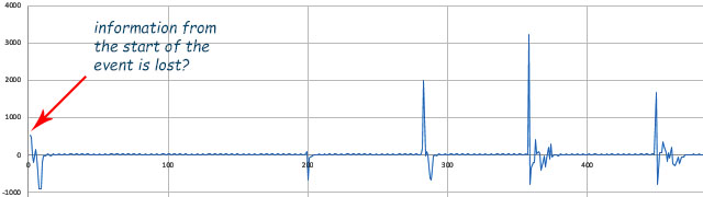
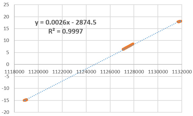
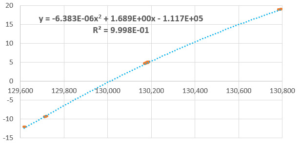
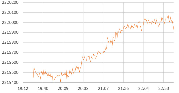
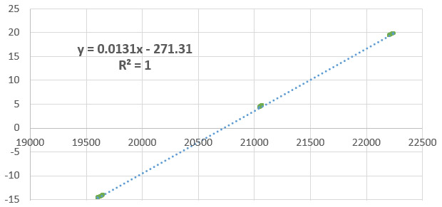
We logged raw single-shot Lux readings at one minute intervals and because there is no averaging applied you can clearly see where overhead lines or birds created occasional short-duration shading. These outliers were excluded before generating the trendline shown below. The PAR values from the model were calculated using the ‘Auto fill’ option for humidity and temperature. On this day solar noon was at 12:57
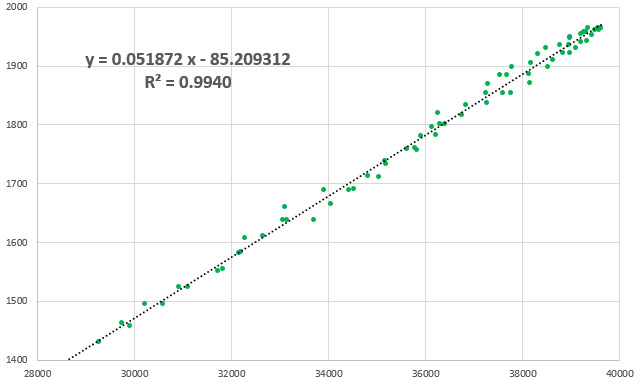
Aerosols and variations in local temp/humidity produced some scatter but this is a good result for calibration with natural light. The result might be improved by co-deploying a humidity sensor, but it’s not clear to me if humidity at ground level is what the model actually uses for its calculation. Some scatter is also being created by the temporal resolution of the model. Using one type of sensor as a proxy for another limits the scope of the device and we probably approached an accuracy of ±15% at best with this conversion. It’s worth remembering that most commercial light sensors are only calibrated to ±5%.
Discussion
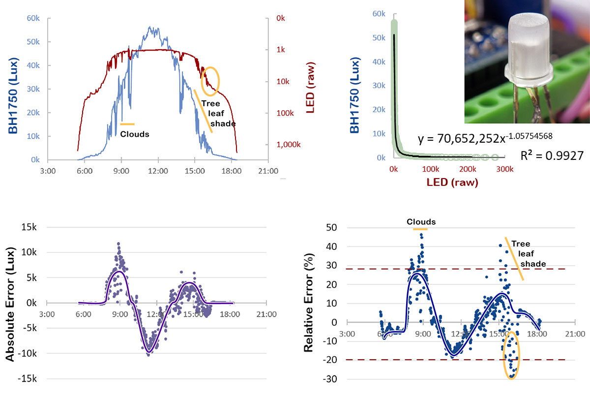
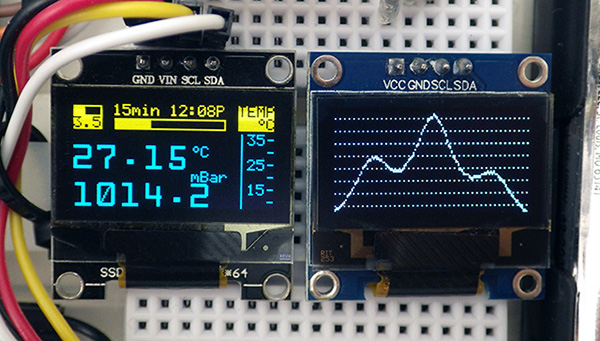
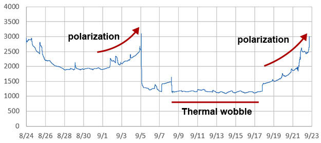
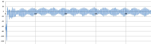
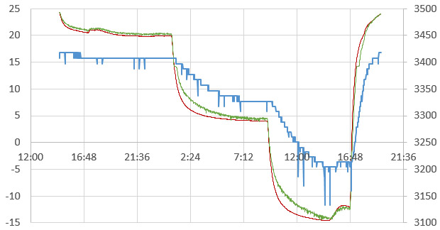
The biggest challenge at our mid-west location was that we had to run the loggers for several weeks before capturing the blue-sky day shown above. Typical time series from that Bh1750 sensor (under a light-reducing diffuser dome) looks like this:
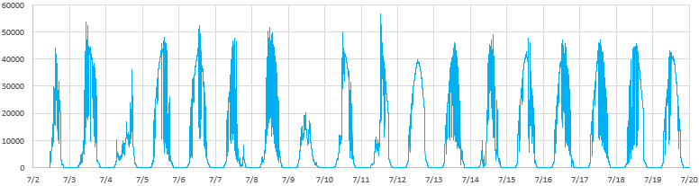
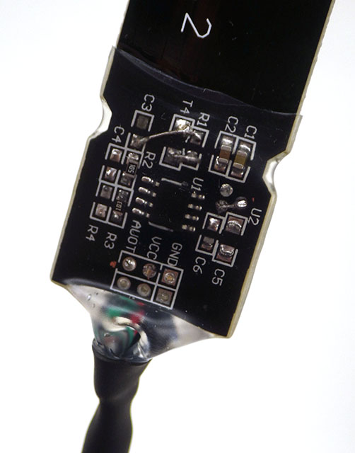
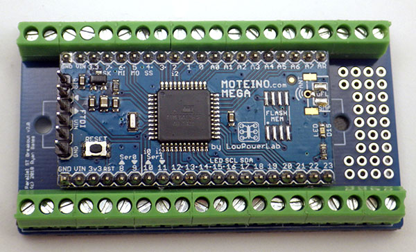
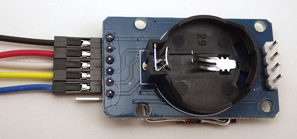
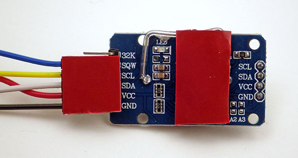
This unit had an extra 64k EEprom added to store the large amount of data that was generated.
Clouds often cause light levels to exceed that seen on clear days. This makes sense if you imagine a situation where there are no clouds directly over-head, but radiation reflected from the sides of clouds is reaching the sensor from multiple directions. The fact that clouds at different atmospheric levels have different effects is one of the things that makes climate models so complicated.
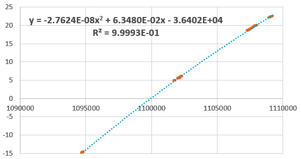
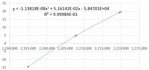
The Clear-Sky Calculator lets you generate data for any date/time, so it would be possible to do this calibration by aggregating cloudless periods from multiple days:

Someone in Nevada would have no trouble gathering this kind of calibration data, but it might not be possible for people living in Washington. A low-cost alternative to using a clear-sky model for the calibration could be to compare the Bh1750 to one of the many smartphone grow light meter apps, with a clip-on diffuser & cosine corrector. Every phone has a different sensor so programs like Photone or PPFDapp usually have their own calibration procedures. While developing this exercise I also found a ‘for parts’ Seaward Solar Survey 100 on eBay for $20, and all it needed to bring it back to life was a good cleaning inside. I also found an old Li-1400 logger with a 190 pyranometer for only $120 and was pleasantly surprised when Apogee’s calculator showed it was still within 5%. As mentioned, you’d need to convert total radiation from those last two into PAR or you could do the calibration to total shortwave. Hardware references that lack logging capability require more effort to gather calibration points, but they save you from having to wait for agreeable weather.
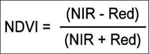
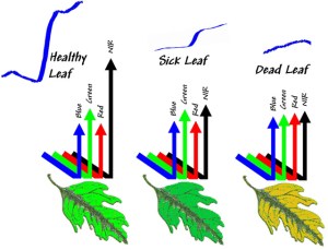
Other projects have built similar sensors and with calibration Lux sensors are comparable to commercial PAR sensors if the spectral environment is consistent. Multi-channel sensors with overlapping frequencies do a better job in situations with discontinuous light sources like those used for indoor growing or for measuring the extinction of PAR frequencies under water. In those cases a TCS3471 (3-channel), AS7341(10-channel), or AS7265 (18-channel) sensor could be used, and finer frequency division can enable calculation of interesting ratios like NDVI or SPAD. Beyond that point you’re entering the realm of diffraction grating spectrometers which allow a more nuanced approach to the spectral function which differs from standard PAR.
And if building your own datalogger is too challenging, you could reproduce the exercise described in this post with a bluetooth UNI-T or a UT381 Digital Luminometer which has some logging capability. But you will need to add extra diffusers to bring full sunlight down below its 20,000 Lux limit.
References & Links
NREL Bird Clear Sky Model
Clear Sky Calculator from Apogee Instruments
NOAA SURFRAD data from irradiance measuring stations
Downloading from the National Solar Radiation Database.
Shortwave Radiation by Steve Klassen & Bruce Bugbee
Fondriest Solar Radiation & Photosynthetically Active Radiation
Designing a Low-Cost Autonomous Pyranometer by Peter van der Burgt
Various DIY PAR meter discussions at Planted Tank
Build Your Own Pyranometer by David Brooks
Ad hoc instrumentation methods in ecological studies produce biased temperature measurements. Terando et al. (2017)
Choosing Standard Bulbs for DIY PAR meter calibration
Daily Light Integral requirements for different plants.
PARbars: Cheap, Easy to Build Ceptometers
DIY Solar Power Meter with an INA226 & solar cell
Creating a Normalized Vegetation Index Sensor with two LEDs
Hacking the Rubisco enzyme boosts crop growth 40%
Plants recycle UV into red light
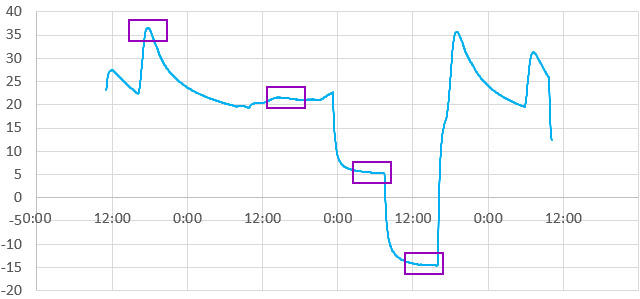
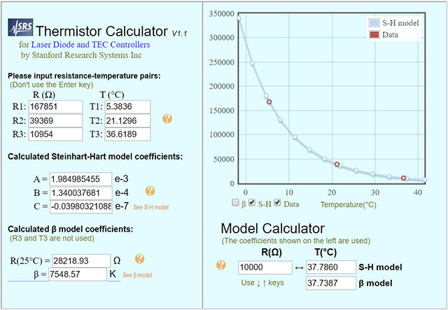
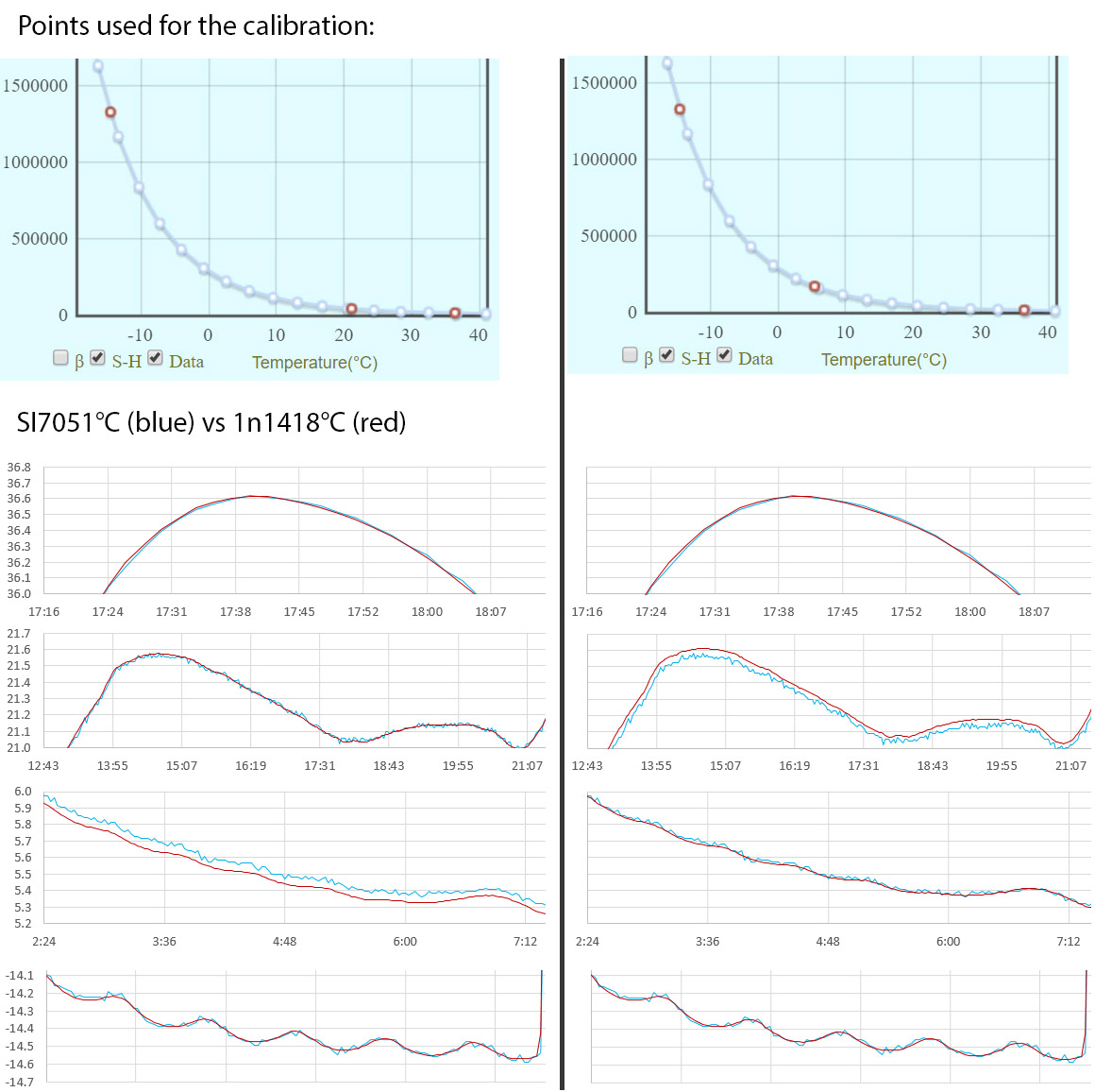
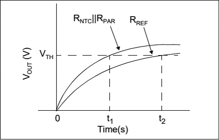
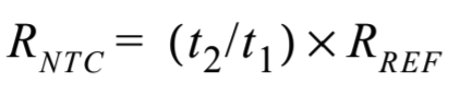
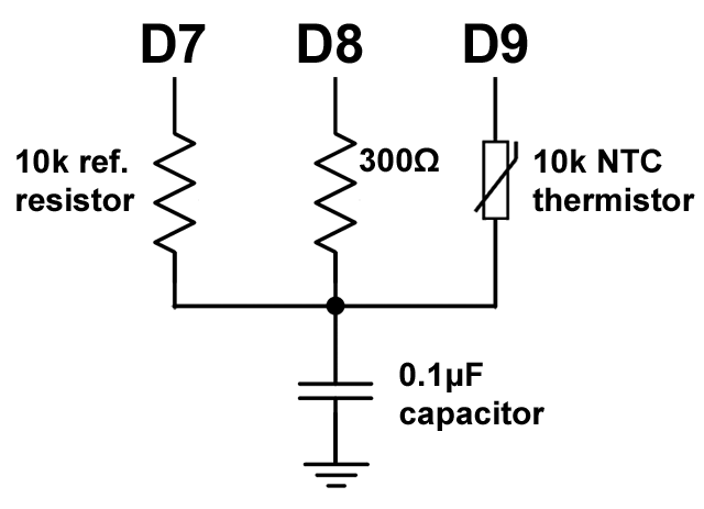
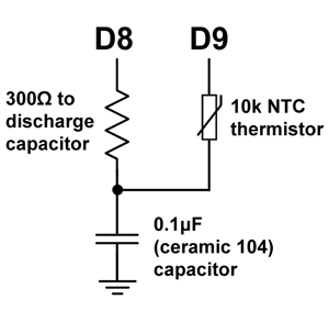
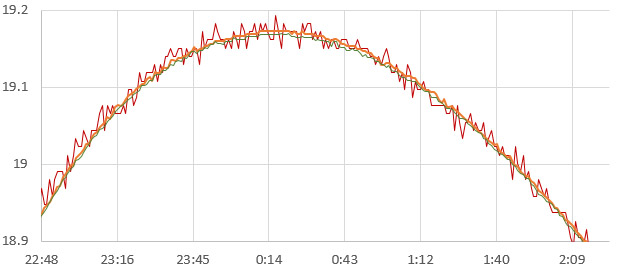
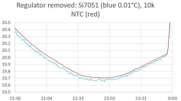
How to calibrate NTC thermistors
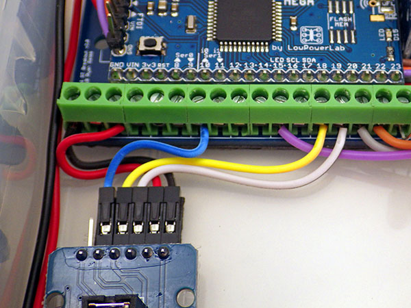
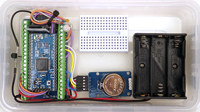
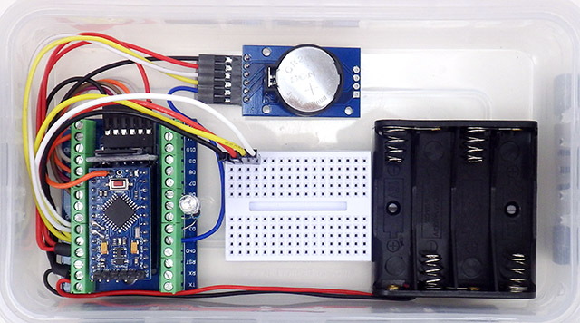
How to build our 2-Part ProMini Data Logger