
Here I’m using a 2019 (v. regulated) classroom logger to create a custom ‘Leaf Transmittance Index’ based on readings from an IR LED and the red channel of the RGB indicator already on the logger. Although using generic LED’s introduces non-optimal aspects wrt frequency & bandwidth, the trial successfully distinguished ‘healthy’ vs ‘unhealthy’ plant leaves where a simple visual inspection could not.
When we released the 2019 version of the classroom logger we updated the starter script to include a technique that uses the indicator LED as a light sensor. This under-appreciated technique leverages the timing capability of microprocessor inputs, rather than the more common approach of using an op-amp to amplify sensor output. Reversing the potential across a diode charges it’s internal capacitance, which can then be discharged by light photons hitting the surface. In ‘reverse bias’ mode, the photon flux is linearly related to the discharge current, however this depletion method changes the voltage across the capacitor at the same time (+ other factors), so we see a response with exponential decay instead of linear.
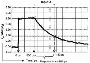
Typical discharge curve for an LED charged up to 5 V and then discharged to a threshold of 1.7 V under artificial lighting (fluorescent tube). Figure 8 from: Absorbance Based Light Emitting Diode Optical Sensors and Sensing Devices pg 2462
Electrically speaking, there is little difference between an LED and a typical photo-diode sensor however an LED’s capacitance is considerably smaller. ( 25 – 60 pF ) The tiny light sensing surface area of an LED (~0.1mm squared) only generates about 50 pA of discharge current in normal ambient conditions, and the reverse leakage through LED’s is exceptionally low (~0.002 pA). The net result is that LED’s are rather slow light detectors, and this phenomenon would be nothing more than a curiosity except for one important aspect: most LEDs detect a relatively narrow band of light wavelengths, making it possible to build a frequency-selective detector without the filters (or monochromators) you’d need to do the same job with photo-diodes or LDRs. That sensitivity band often has less drift over time than many types of filters and the discharge/photocurrent method has less temperature dependence than using the same LED in photovoltaic mode.
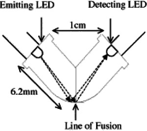
Illustration from that same Sensors review paper, but originally from: Novel fused-LEDs devices as optical sensors for colorimetric analysis. Talanta 2004, 63, 167–173. Sometimes these these emitter-receiver pairs are dip coated with a chemo-reactive membrane. Their next paper: Quantitative colorimetric analysis of dye mixtures using an optical photometer based on LED array Sensors and Actuators (2006), used a series of different emitter LEDs and a low band gap IR LED as a universal light detector. Xiao et al in 2009 used blue excitation LED’s that match the excitation wavelengths of common fluorescent dyes like fluorescein.
This makes a host of new LED-based instruments possible at the DIY level, and Forest Mims demonstrated this with some elegant experiments using near-IR LEDs detecting atmospheric water vapor, aerosols with twilight photometers, and he even proved that a single red LED reading provides a reasonable proxy for total PAR. (using a red gallium phosphide (GaP) LED with a wide (115 nm FWHM) absorption band @ 600-655 nm) Since Mim’s pioneering work in 1977, the number of applications for LED sensors has grown so fast that now it’s hard to keep up with the ‘review papers’, let alone the individual publications. Bench-top chemistry is seeing a host of fluorescence & reaction cell experiments based on frequency matched LED emitter-detector pairs. By rapidly toggling the same LED between emitting and detecting light, several projects have created other types of sensors like ocean PH. We can only imagine what will happen when up-converting nanoparticles get thrown into that mix.
What can we do with our logger
using this LED measurement technique?

Here a day of raw readings from all three LED channels are compared to an LDR in same classroom logger. The unit was deployed in a south facing window with diffusing tape over the housing surface.
Light detectors are often used to make measurements of energy balance, usually by tracking solar insulation. Using the RGB indicator LED already on the logger means we only have a limited number of light frequencies to work with, so we can’t create a ‘full spectrum’ pyranometer unless we use a more advanced solution like SparkFun’s Triad Spectroscopy Sensor . Combining that with good mounting bracket , would provide enough frequency coverage to match some commercial instruments.
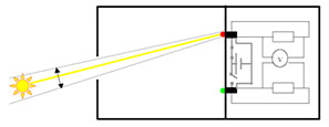
Figure 2.1. LED-based Sun photometer for the GLOBE project. The rectangles with the green (505nm) and red (625nm) spheres represent the LEDs. From The Contribution of Dutch GLOBE Schools to Validation of Aerosol Measurements from Space
Despite this limitation, a few dedicated groups have proven that LED photometers can still be quite capable. Most notably the 2-LED Globe program photometers by Brooks et al. at the Institute for Earth Science Research and Education It is quite inspiring to see students using hand-made instruments to produce research good enough to publish in peer-reviewed journals.
The Globe device uses a more traditional op-amp approach to reading the LEDs, but several aspects of those instruments are directly transferable to other light-sensing projects:
- LED sensors are exceptionally stable over time.
- Students can manually aim the detectors at the sun, enabling a basic instrument to do the work of more complicated “sun tracking” machines that use directional control, collimators or shadow bands to measure diffuse irradiance. From Mims PAR paper: “Measurements are made each day at or near local solar noon when the solar disk is not obscured by clouds. Measurements are made by placing the radiometer on a level platform 175 cm above an open grass field. Two measurements are made of each channel; first the full sky and then the diffuse sky. The latter measurement is made when the diffuser of the sensor is shaded by a 19 mm diameter disk mounted on a rod.”
- Two or more measurements are needed because it’s the difference between those readings that allows you to derive the property you were trying to measure. For example, if you had two diodes, with one responding to UV-a and the other responding to UV-b, the difference between those readings could be attributed to atmospheric ozone. Comparing readings from two IR sensors with one at the 940nm H20 absorption peak and another sensor at 890nm, would let you derive water content.
- This also requires correcting for scattering/absorbance by the atmosphere ( Path Length = 1/cos(θ) ) based on the suns angle in the sky (also note: many diy PAR projects hack the white plastic domes out of old photometers as cheap cosine correctors.) Better instruments also correct the ~1% / °C temperature coefficient of red spectrum LEDs, which is higher than that of silicone photodiodes.
- The biggest challenge is determining unique the absorption band of the LED you are working with since that information is not supplied by manufacturers. The process usually requires testing the LED(s) with a wavelength scanning monochromatic light source.
All of Forest Mims LED-based experiments could be replicated with the Cave Pearl classroom logger using the capacitance discharge timing method instead of using an op-amp for current to voltage translation. But there’s a more information to be had from LED-sensors by anyone willing to do a little tinkering, especially in the area of vegetation monitoring.
Spectral Characteristics of Vegetation:
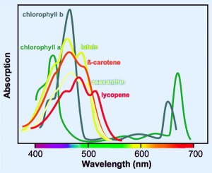
Note photosynthesis has a relatively absorption-free range: 550-630nm. to protect the plants from oversaturation damage.
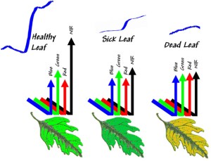
Photosynthetic pigments absorb significant amounts of the red and blue light falling on healthy vegetation. Many papers focus on chlorophyll, but there are several other ‘antenna pigments’ which also absorb light to enhance photosynthetic efficiency. Approximately half of the un-absorbed visible radiation is reflected, leading to the green appearance of leaves. Reflectance is much higher at near infrared (NIR) frequencies than in the visible region due to the cellular structures inside the leaves.
Normalized Vegetation Indexes:
A friend recently sent me a link to Rick Shory’s extensive work on the greenlogger which hit the in-box around the same time as SciAm’s article: Earth Stopped Getting Greener 20 Years Ago. Reading about the global decline in vegetation set me on a deep dive into how indexes are used in bio-physical monitoring:
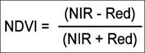 NDVI was developed to estimate vegetation cover from remote sensing data. It is calculated from red and NIR spectral reflectance measurements, and the first key understanding is that spectral reflectances are normalized ratios of the reflected over the incoming radiation in each spectral band. Feeding those ratios into the NDVI calculation means that it can only produce values between -1 to +1.
The second key understanding is that using the ratio of the difference of the red & infrared over their sum corrects for the effect of the solar zenith angle. This eliminates irradiance from the equation, and largely corrects for differences due to topography and transmittance loss in the atmosphere. This allows the comparison of remote sensing data from different times of day, and different latitudes.
NASA uses NDVI as a an indicator of drought, When water limits vegetation growth, it has a different relative NDVI than when the same plant is hydrated because the spongy mesophyll layer deteriorates, and the plant absorbs more of that near-infrared light rather than reflecting it. This is a significant factor for agricultural yield prediction..
Moderate NDVI values represent low density of vegetation (0.1 to 0.3), while high values indicate dense vegetation (0.6 to 0.8) Zero indicates the water cover, and lower values of NDVI (-0.1 and below) correspond to barren areas of rock, sand, or urban/built-up. In addition to land cover classification, people use NDVI to infer parameters like Leaf Area Index (LAI), fractional light interception (fPAR), wildfire burn-area, and other aspects of the biological environment. But the NDVI index also has some limitations: Any time there’s very low vegetation cover (majority of the scene is bare earth), NDVI will be sensitive to that soil. On the other extreme, where there’s a large amount of vegetation, NDVI tends to saturate.
Over time NDVI has been tweaked in various ways and today there are a large number of different Broadband ‘Greenness’ Indexes that accent different aspects of plant physiology. And the booming agricultural drone business seems to be inventing more by the day, with claims that somehow their camera tweak produces a new index that’s superior to those of it’s competitors, while their competitors make equally strident claims that company #1 doesn’t know what they are talking about. Public lab has an active community of people hacking cameras for this kind of imagery.
Can we use the RGB LED on the Classroom logger to measure a Vegetation index?

Fig.4.24, pg49, Approximated Emission and Sensitivity Spectra (of an OSRAM LH-W5AM RGB led) from: Using an LED as a Sensor and Visible Light Communication Device in a Smart Illumination System, Dissertation by André Filipe Rato Bispo
The first challenge is figuring out what we can actually detect, since each index works with a given set of frequencies. An LED will only detect light with higher energy photons than the light it emits, so a blue LED will be unable to detect red frequencies. LEDs generally have peak detection capability 20-60nm shorter than the wavelength they emit with the range widening, but this information is rarely available from manufacturers because it’s a use case they were never designed for. So there are not many sources that compare the emission and detection frequencies for the different LED chemistries. LEDs: Sources and Intrinsically Bandwidth-Limited Detectors (Figure 5) has a reasonable list of specific LEDs characterized as both sources and detectors, but even they didn’t bother to test a garden variety RGB. Fortunately a few researchers working on visible light communication projects have tested them, generally finding that the blue emitter shifts into UV-A 320-400 nm detection range (possibly near one of the UV-A peaks of the phototropic action spectrum?) , the green emitter shifts down to about 440-460 nm (detecting in chlorophyll a/b blue absorption bands?), and the red LED channel shifts down to ~680nm, with a spectral spread 2 to 3 times wider than its emission band. (overlaps the chlorophyll a red absorption peak?).
Testing to see how a 488nm dichroic mirror (blue cut-off filter) affected readings on the Green LED detection channel. Note that in this case the round lens was also removed from the top of the LED with sandpaper to both collumnate and diffuse the incoming light. But with the PTFE tape layer added later, the sanding was unnecessary for the index measurements.
But was this true for my LED? Since we didn’t have a “wavelength scanning monochromator” just lying around I tested the green channel with a blue-cutoff Dichroic Mirror Unlike regular filters, dichroic mirrors are intended to work only for incoming light that is normal to their surface – but given the tight 20 degree dispersion angle of typical 5mm leds, that’s probably OK. If I was looking for a range of different filters on the cheap, I’d probably look at safety glasses designed for laser work – they usually come with a well specified transmission curves & very sharp cut-offs at certain frequencies.
Sure enough, the discharge on the ‘blue-shifted’ green channel took more than 10x longer with the filter in place, indicating that the green channel was sensitive to frequencies below the filters 488nm cut-off. If the red LED channel also follows the pattern from Bipso’s paper, then red’s detection will include some green & some red, with a peak at yellow. We might be able to use these frequencies for a BLUE vs GREEN variant of NDVI, but several sources indicating that blue indexes were sub-optimal because that chlorophyll absorption is strongly overlapped by carotene. So blue based indexes usually show less contrast between stressed versus non-stressed plants. The loss of both the blue channel (now a UV detector) and the green channel (now a blue detector) meant that we need to add an IR led to have enough information for a viable index.
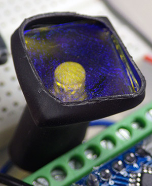
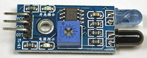
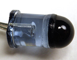
IR obstacle avoidance modules are one inexpensive source of IR LEDs. These sensors are somewhat limited when used for their intended purpose, but a little cut & paste lets you merge the emitter LED with a daylight filter ‘cap’ cut from the photo-transistor on the same board:
 |
 |
 |
IR detectors can be sensitive to visible light unless you add a daylight filter, and this little hack is much cheaper than buying a Wratten 87, 87B, or 87C. These distance modules usually have LEDs which emit at 940nm, but the same shorter wavelength-shift also applies to the IR LED, and this pulls the detection peak into the 920nm range – safely out of the absorbance well created by atmospheric water vapor(?). (something to keep in mind if you are actually trying to build a water vapor sensor – you probably need to select an emitter at least 25 nm above 940)
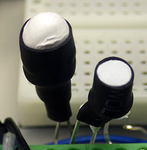
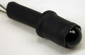
Note that the negative terminal of the IR LED is under the same screw terminal (D7) as the common cathode leg of the RGB indicator led. Columnating the LEDs with heat shrink tubing should also make them less sensitive to light reflections inside the logger. Note: our GitHub code uses a port command that assumes that shared ‘negative’ pin to be one of D3 to D7 on the pro mini. Here I’ve set #define LED_GROUND_PIN 7 as the common GND connection, RED_PIN 6, GREEN_PIN 5, and the positive side of the IR led is on pin D8. Set #define BLUE_PIN 8 to force the former blue pin code to take the IR LED reading. Also note: that our code initially ‘lights’ the indicator LED via INPUT_PULLUP mode, instead of setting the pins to OUTPUT & HIGH, so limiting resistors are not necessary for that step.
Even with a filter and heat shrink tubing the IR LED was easily saturated, and it took 28 layers of plumbers tape to bring readings from the IR LED into approximately the same range as the RGB readings (which had only 1 layer of diffusing PTFE tape on it) This was done with the logger tethered a laptop, displaying readings in the serial monitor window. I simply added one layer at a time until the readings under direct full sunshine for both the IR & Red channel were in the 300 to 500 range (using our logger code from Github). Then I add some heat shrink to hold those layers of teflon tape in place, leaving only the round dome of the LED(s) exposed.
Even with IR on board, the lack of a sharp red detector means we can’t produce the traditional NDVI. (unless we add a Wratten25) With the ‘red’ LED channel actually detecting from 525 to 650 (FWHM 560-610) and peaking around 575nm we have to invent our own pseudo index that might be described as ‘lime-green’ NDVI. This actually isn’t so bad, as several recent papers demonstrate that green-based NDVIs are more sensitive to chlorophyll than the red based indexes, and they have stronger correlation with total leaf area. (It’s also worth noting how close we are to the bands typically used for pulse oximetry, where the reading from a red LED at 600nm is ratioed with a second measurement from an IR-LED responding at 950nm)
Other Challenges:
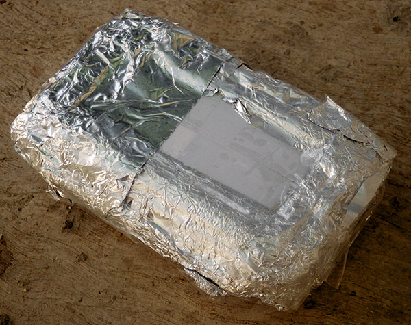
With a tinfoil wrap, light can only enter through the 5 x 8cm exposure window above the LEDs. One layer of blank label-maker tape on the lid diffuses the light and prevents the plastic struts inside the housing from creating hot-spots. A final outer wrap of clear packing tape protects the tinfoil.
Bandgap voltages vary with temperature, changing the LED emission wavelength by ~ 0.1nm/°C. Detection wavelengths should follow suit, so it’s probably best to make sure the temperature varies as little as possible between our scale points and the target readings. Since the LED detectors are inside a Plano box, there is potential for some frequencies to be lost, but materials like high density polyethylene (HDPE) have remarkably smooth absorption curves that don’t become extreme until you reach UV. The fact that Vi’s are ‘a ratio of ratios’ means that we have to compare the raw sensor readings to direct insulation values before the index can be calculated. Housing losses should affect the high reference and the target readings in the same way, so it should not throw off the final index – essentially we treat it like transmittance loss in the atmosphere. And I need to use a desiccant because this is a capacitance – discharge method, so things like ambient humidity could affect the capacitance.
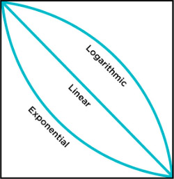 Since we can’t know the responsivity of our garden variety LEDs without lab testing, the best we can do is standardize the data by scaling it against a “maximum” reading (when the sun is shining directly on the top of the logger) and a second “minimum” point for each channel (obtained by covering the entire logger with tinfoil). The dark point reading also address thermal leakage through the LEDs. One drawback of this mcu-based method is that the raw discharge-time readings follow an exponential decay curve, so we need to take the log of those readings to linearize the data before scaling, and since our decay-time readings are inversely related to the photon flux, we need to apply 1/LN(reading) to all data before the max/min scaling. Technically speaking, photon flux is not the same as irradiance, but the the index’s normalization sweeps that little issue under the rug too.
Using the sun as our high scale point necessitates that the readings are done under a clear blue sky. Clouds passing overhead between readings (or other haze / humidity variations) could change the ratio of IR to visible light more than the plants you are trying to monitor: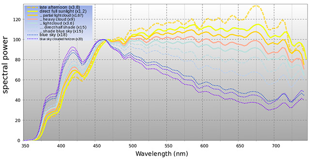
Rain is another potential complication, as water strongly absorbs IR. So the readings have to be taken long enough after a rainfall that no water droplets are present on the surfaces. So with the basic 2x LED configuration I’m using here, you have to wait for good weather, and take the readings under a clear blue sky, between mid morning & mid afternoon.
Cloud induced variations could be compensated by putting two sets of sensors on the logger (one pointing up & one pointing down) for simultaneous correction of direct insolation vs surface reflectance, but for now this is just a prototype trial to see if a decent ‘lab exercise’ can be developed for the Cave Pearl Loggers with minimal additions to the basic build.
Does it work?
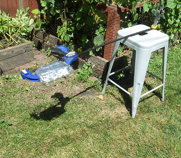
Backyard trial testing the reflectivity of my lawn in an area deliberately chosen as “unhealthy” grass .
With all the rough assumptions up to this point I was surprised to find the reflectance readings falling within the broad range of ‘textbook’ values. A reading 1m above a relatively healthy section of my lawn produced an index of 0.39 while a reading above a mangy half-dead section (photo: right) produced a much lower index value around 0.215 A patch of bare dirt read at 0.044, and my gravel driveway produced an index of -0.13 The front flower garden produced a reading of 0.292 It’s hard to know how representative this is given the wide range of values listed for different plant species in the various spectral libraries.
With the challenges of species variation & water condition, the use of verified bright & dark targets is pretty common in biophysical sensing. White panels coated with barium sulfate paint, Komatex, or Teflon are sometimes used because they have reflectance near 100% with very few specular artifacts. NASA’s Aster Spectral Library suggests that most flat black paints have a similar response through visible and NIR, so some Rustoleum on a big sheet of cardboard might work as a 4% calibration point.
A better idea for the classroom:
Covering large areas with a grid of these single-shot readings would take a substantial amount of time, and even relatively short trials run into issues with trees and other large shadows creeping into the test patches throughout the day. So logging reflectance is more suited to long-term measurements of vegetation cover at single location. (or forest canopy transmittance)
After a bit more reading, I began to notice a pattern:
![]()
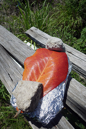
(click to enlarge) Leaves cover the input window, secured to prevent wind shifting.
So index calculations ought to work with light that is transmitted through the leaves because the two curves contain very similar information. With the standard reflectance-based NDVI, ratings between 0 and 0.33 indicate unhealthy or stressed plants, 0.33 to 0.66 is moderately healthy, and 0.66 to 1 is very healthy. Flipping the calculation to a transmission-based version will shift those values significantly, but we can still use that trend as a rough guide to whether the method is working.
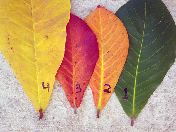
As luck would have it, this insight occurred just before another fieldwork trip, so it was more than a week before I could test the idea. The first trials used leaves from tropical almond trees which are dry-season deciduous. Re-capturing some of their ‘energetically expensive’ chlorophyll turns the leaves pinkish-red or yellow-brown due to the leftover pigments such as violaxanthin, lutein, and zeaxanthin. These Xanthophylls are yellow pigments from one of the two major divisions of the carotenoid group (the other division is formed by the carotenes). They act to modulate light energy and may also serve as a non-photochemical quenching agents to deal with excited states of chlorophyll that are overproduced during photosynthesis under the intense light conditions.
 |
|||
| Leaf Number | Red RGB channel: scaled % of full sun reading |
IR LED reading: scaled % of full-sun reading |
(gYr) “Transmission based” NDVI |
| #1 (green) | 37.24 | 82.81 | 0.380 |
| #2 (orange) | 59.47 | 83.13 | 0.166 |
| #3 (red) | 42.22 | 80.95 | 0.314 |
| #4 (yellow) | 67.62 | 82.91 | 0.102 |
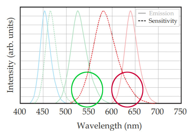
The overlap of the sub-LEDs at 550nm is leveraged for transmission (green) and photodetection (red) in short range visible light communications.
All leaves were ‘fresh-picked’ from the tree, and the percent transmission numbers were averaged from five readings taken one minute apart. Natural light is notoriously variable, so most index sensors use considerably more sample averaging than that.
It’s not surprising that the yellow leaf was well discriminated, but the fact that the green & red leaves produced similar values highlights an issue with our rough prototype: the widened spectral spread of the red LED channel makes it difficult to distinguish between light frequencies on either side of the response curve.
 |
 |
 |
 |
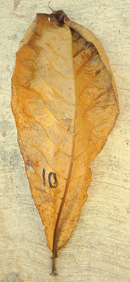
| Leaf (click to enlarge) | Red RGB channel: scaled % of full sun reading |
IR LED reading: scaled % of full-sun read |
(gYr) T-NDVI |
| #10 (Dead on ground) | 26.96 | 65.38 | 0.416 |
| #11 (yellow patch) | 44.90 | 79.45 | 0.278 |
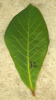
| #12 (green & healthy) | 34.27 | 76.17 | 0.379 |
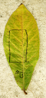
| #13 (>50% yellow) | 55.56 | 77.79 | 0.167 |
Despite the limited red/green selectivity, this set shows that, at least for ‘fresh’ leaves, our custom index can still discriminate the loss of the chlorophyll. The dead leaf suggests that will only work up to a point. Dead vegetation reflects a greater amount of energy than healthy vegetation throughout the visible spectrum but reflects less IR, so any actual ‘dead-spots’ will raise a transmission-based index value. This is a limitation for our method – which does not produce a natural separation between healthy and dead vegetation like a reflectance based index would. This would be serious problem for remote sensing applications, but when a leaf that you can hold in your hand is that badly off, you probably don’t need a sensor to tell you the plant is not thriving.
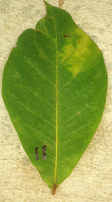
Does this transfer to other plant species?
 |
 |
 |
 |
| Leaf (click to enlarge) | Red RGB channel: scaled % of full sun |
IR LED reading: scaled % of full-sun read |
(gYr) T-NDVI |
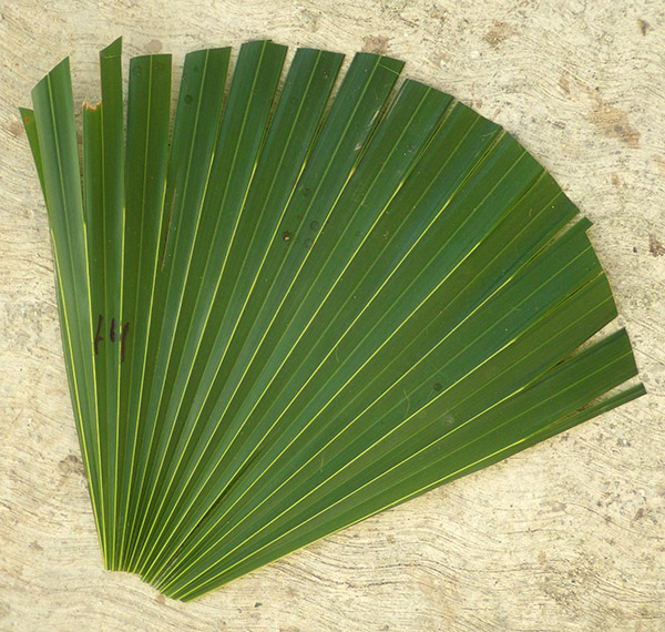
| #14 (Green leaf – from stressed plant1) |
39.29 | 77.51 | 0.327 |
| #15 (Brown spots – from stressed plant1) | 37.71 | 76.23 | 0.338 |
| #16 (Green leaf from healthy plant2) |
21.83 | 68.05 | 0.514 |
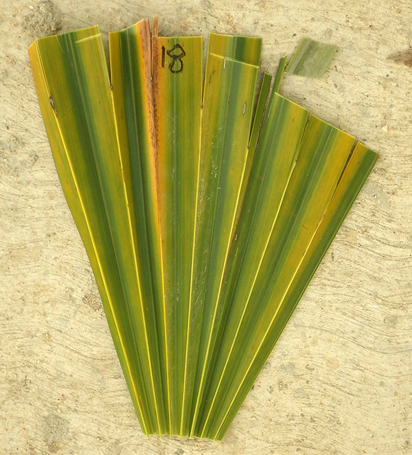
| #18 (>50% yellow – other stressed plant3) | 32.65 | 65.47 | 0.334 |
As expected, the overall light transmission numbers were different for palm than they were for the tropical almond leaves. So a calibration set would need to be created for each plant species to put these numbers into context. I’m assuming the green/yellow discrimination is due to chlorophyll levels in the almond leaves, but there could be other confounding factors like Anthocyanin in the hardier palm leaves. (Antho. also absorbs in our sensor band, and is abundant in senescing leaves)
While #14 and #15 look different they were taken from same plant, and the yellow-brown spots on #15 make it clear the plant was under some kind of stress. Visually, I would not have been able to distinguish leaf #14 from #16 but the index identified #14 as being from an “unhealthy” plant. Given the relatively wide spectrum we are working with here, this is a remarkable result – suggesting that with a bit of homework to find LED’s with tighter detection bands, we could produce an inexpensive chlorophyll meter (like the SPAD?) or we could tune the idea for other pigments/applications. It should be possible to at least match the performance of the leaf color charts currently being used to assess when fertilizer is needed. Using a white LED emitter above the leaf could enable a variant of our simple approach that was not dependent on the sun, and adding couple of reads using only green & red emitters above the leaf would enable us to distinguish which side of that wide detection curve we were on. Commercial chlorophyll meters sometimes use emitters at 660 nm & 940 nm , measuring both reflectance AND transmission so an accurate absorbance value can be calculated. Even then plants cease to create chlorophyll once a certain threshold has been reached, so these meters are often used to detect deficiencies (by comparison to a well fertilized control group) rather than concentrations.
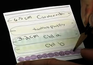 And finally, a classroom lab could combine this kind of index-based characterization with paper chromatography to verify the pigments in the leaves via their Rf factors. A more advanced approach would do this quantitatively, turning this index into a true diagnostic tool. This could also be a good accompaniment to the many other Arduino based plant monitoring projects, as a growth or health verification stage. In northern climates this could even be done with house plants by taking readings ‘before’ and ‘after’ some experimental intervention. With those large temporal separations, you would want to take new max/min readings each time for the scaling & avoid using artificial light sources as these introduce frequency artifacts that could interfere with the index.
Addendum (2020-10-28): Oxygenated hemoglobin with LED sensors
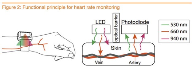
“The same procedure is used for oxygen saturation measurement. Here the principle is to measure the absorption of the hemoglobin in the blood. Oxygenated hemoglobin (HbO2) has a significantly different absorption of light than non-oxygenated hemoglobin (Hb). To detect this difference, the skin is illuminated with one red and one IR LED light and a photodetector measures the absorption.”
Addendum (2024-08-10): Measuring PAR with Bh1750 Lux sensors

Readers of this post might also enjoy the tutorial we developed on how to cross-calibrate a Bh1750 lux sensor to measure PAR (Photosynthetically Active Radiation). This was done with natural sunlight and a clear sky model calculation, which provided some challenges. But there are many alternative references that could be used, and the most important aspect of the procedure was the mechanism we created for leveling the sensors – which is absolutely required. I also found another paper that characterizes some single-color LEDs as photodetectors.

Pingback: Creating a ‘Plant Health’ tester with two LEDs – Arduino Apprentices
Pingback: The Cave Pearl Project's Edward Mallon Showcases Accurate Temperature Sensing with a Single Diode • beat 10z