
We’ve been using a reverse bias discharge technique to turn the indicator LEDs on our loggers into light (& temperature) sensors for several years. The starter code on GitHub demonstrates the basic method but as the efficiency of garden variety RGBs continues to improve, I’ve noticed that the new ‘super-bright’s also seem to photo-discharge more rapidly than older LEDs. Sometimes the red channel discharges so quickly that we hit the limit of that simple loop-counting method with our 8Mhz processors.
Normally when I want more precise timing, I use the Input Capture Unit (ICU) which takes a snapshot of the timer1 register the moment an event occurs. This is now our preferred way to read thermistors, but that means on most of our deployed loggers the ICU on D8 is already spoken for. And a multi-color LED offers interesting ratio-metric possibilities if you measure each channel separately. That prompted me to look into PIN CHANGE interrupts, and I’m happy to report that, with a few tweaks to suspend other interrupt sources, Pin Change & Timer1 can approach the limits of your system clock. So results are on par with the ICU, but Pin Change extends that ability to every I/O line. With slow sensors, where the counts are high, I usually put the system into sleep mode IDLE to save battery power while counting, but that adds another 6-8 clock cycles of jitter. Sleep modes like power_down are not used because the ~16,000 clock cycles that the processor waits for oscilator stabilization after deep sleeps makes accurate timing impossible.
If you are new to interrupts then Nick Gammons interrupt page is definitely the place to start. (seriously, read that first, then come back & continue here…) The thing that makes working with interrupts complicated is that microcontrollers are cobbled together from pre-existing chips, and then wires are routed inside the package to connect the various ‘functional parts’ to each other and to leads outside the black epoxy brick. Each ‘internal peripheral’ uses a memory register to control whether it is connected (1) or not (0) and several sub-systems are usually connected to the same physical wires. Each of those ‘control bits’ have names which are completely unrelated to the pin labels you see on the Arduino. So you end up with a confusing situation where a given I/O line is referenced with ‘named bits’ in the GPIO register, and other ‘named bits’ in the interrupt peripheral register, and yet more ‘named bits’ in the ADC register, etc. Pin Maps try to make it clear what’s connected where but even with those in hand it always takes a couple of hours of noodling to get the details right. I’m not going to delve into that or this post would scroll on forever, but there are good refs out there to Googlize.
Fast Reading of LED light sensors:
#include <avr/power.h>
#define RED_PIN 4 // my typical indicator LED connections
#define GREEN_PIN 6
#define BLUE_PIN 7
#define LED_GROUND_PIN 5 //common cathode on D5
volatile unsigned long timer1overflowCount;
// Reading the red channel as a stand alone function:
uint32_t readRedPinDischarge_Timer1() {
// discharge ALL channels by lighting them briefly before the reading
digitalWrite(LED_GROUND_PIN,LOW); pinMode(LED_GROUND_PIN,OUTPUT);
pinMode(BLUE_PIN,INPUT_PULLUP); pinMode(GREEN_PIN,INPUT_PULLUP);
pinMode(RED_PIN,INPUT_PULLUP);
//execution time here also serves as the LED discharge time
byte gndPin =(1 << LED_GROUND_PIN);
byte keep_ADCSRA=ADCSRA;ADCSRA=0; byte keep_SPCR=SPCR;
power_all_disable(); // stops All TIMERS, save power and reduce spurious interrupts
bitSet(ACSR,ACD); // disables the analog comparator
digitalWrite(BLUE_PIN, LOW);digitalWrite(GREEN_PIN, LOW);
digitalWrite(RED_PIN, LOW); //end of the LED discharge stage
//reverse prolarity to charge the red channels internal capacitance:
pinMode(RED_PIN, OUTPUT); pinMode(LED_GROUND_PIN, INPUT_PULLUP);
_delay_us(24); //alternative to delayMicroseconds() that does not need timer0
noInterrupts();
// enable pin change interrupts on the D5 ground line
bitSet(PCMSK2,PCINT21); // set Pin Change Mask Register to respond only to D5
bitSet(PCIFR,PCIF2); // clears any outstanding Pin Change interrupts (from PortD)
bitSet(PCICR,PCIE2); // enable PinChange interrupts for portD ( D0 to D7 )
set_sleep_mode (SLEEP_MODE_IDLE); // this mode leaves Timer1 running
timer1overflowCount = 0; // zero our T1 overflow counter
// reset & start timer1
TCCR1A = 0; // Compare mode bits & wave generation bits set to zero (default)
TCCR1B = 0; // Stop timer1 by setting Clock input Select bits to zero (default)
TCNT1 = 0; // reset the Timer1 ‘count register’ to zero
bitSet(TIMSK1,TOIE1); // enable Timer1 overflow Interrupt so we can count them
bitSet(TCCR1B,CS10); // starts timer1 prescaler counting @ 8mHz (on 3v ProMini)
interrupts();
PIND = gndPin; // faster equivalent of digitalWrite(LED_GROUND_PIN,LOW);
do{
sleep_cpu();
}while ( PIND & gndPin ); //evaluates true as long as gndPin is HIGH
TCCR1B = 0; // STOPs timer1 (this redundant – but just making sure)
bitClear(TIMSK1,TOIE1); // T1 Overflow Interrupt also disabled
sleep_disable();
bitClear (PCIFR, PCIE2); // now disable the pin change interrupts (D0 to D7)
bitClear (PCMSK2,PCINT21); // reset the PC Mask Register so we no longer listen to D5
bitSet (PCIFR, PCIF2); // clear any outstanding pin change interrupt flags
power_timer0_enable(); // re-enable the peripherals
power_twi_enable();
power_spi_enable(); SPCR=keep_SPCR;
power_adc_enable(); ADCSRA = keep_ADCSRA;
power_usart0_enable();
pinMode(RED_PIN,INPUT);
pinMode(LED_GROUND_PIN,OUTPUT); // normal ‘ground’ pin function for indicator LED
return ((timer1overflowCount << 16) + TCNT1);
//returning this as uint32_t, so max allowed is 4,294,967,295
}
// and the required ISR’s
ISR (TIMER1_OVF_vect) {
timer1overflowCount++;
if(timer1overflowCount>10000){ // this low light limiter must be <65534
DDRD |= (_BV(LED_GROUND_PIN)); // sets our gnd/D5 pin to output (is already LOW)
// Bringing D5 low breaks out of the main do-while loop
TCCR1B = 0; // STOPs timer1 //CS12-CS11-CS10 = 0-0-0 = clock source is removed
}
}
ISR (PCINT2_vect) { // pin change interrupt vector (for D0 to D7)
TCCR1B = 0; // STOPs timer1
DDRD |= (_BV(LED_GROUND_PIN)); // forces GND pin low to break out of the sleep loop
}
Key details:
The code above tweaks our standard discharge method (on GitHub) with port commands & PIND when things need to happen as fast as possible, but also uses slower digitalWrite/pinMode commands in places where you want to spend more time ( in the pre-read channel discharge steps ). The power register lowers current draw during SLEEP_MODE_IDLE, but power_all_disable(); also shuts down Timer0, so those pesky 1msec overflows don’t disturb the count. Waking from SLEEP_IDLE adds a constant offset of about 8 clock cycles , but it reduces the jitter you’d normally see with the CPU running. One or two clock cycles of jitter is normally unavoidable with a running processor because you can’t respond to an interrupt flag in the middle of an instruction. Interrupts are also blocked when you are processing some other interrupt, so if the AVR is dealing with a timer0 overflow – the LED triggered pin change would have to wait in line.
This Timer1 method increases resolution by an order of magnitude (so you can measure higher light levels) but that lead me to the realization timing jitter is not the major source of error in this system. Before light even reaches the diode it is redirected by the LED’s reflective cavity and the encapsulating lens. Sampling time is also a factor during calibration because light levels can change instantaneously, so any temporal offsets between your reference and your LED reading will also add noise.
Does light sensing with LEDs really work?
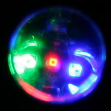
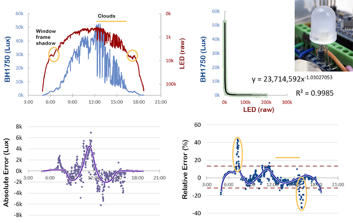
One way to demonstrate the limits of a garden variety RGB is to cross-calibrate against the kind of LUX sensors already in common use. Most LED manufacturers don’t worry much about standardizing these ‘penny parts’, so {insert here} all the standard quid pro quos about the limitations of empirically derived constants. I covered frequency shift in the index-sensor post, and there’s an obvious mismatch between the wide spectral range of a BH1750 (Lux sensor) and the sensitivity band of our LED’s red channel:


Most of us don’t have a benchtop source to play with so I’m going try this using sunlight. The variability of natural light is challenging, and the only thing that lets me use that LED band as a proxy for LUX is that intensity from 400-700nm is relatively consistent at the earths surface.

The most difficult lighting conditions to work with are partially cloudy days with many transitions from shadow to full sun. Because the reference and LED sensors are in different physical locations within the housing shadows that cross the logger as the sun moves across the sky will darken one of the two sensors before the other if they are not aligned on the same north-to-south axis before your tests.
Skylight also undergoes a substantial redistribution of frequencies at sunrise/sunset and that may produce a separation between the response of the ‘yellow-green’ sensitive red LED channel, and the wider sensitivity range of the BH1750.
The biggest challenge for a cross calibration is that LEDs don’t match the ‘Lambertian’ response of our reference. A bare silicon cell has a near perfect cosine response (as do all diffuse planar surfaces) producing a perfectly spherical pattern on polar intensity diagrams. The BH1750 comes very close to that, but LED’s have a range of different patterns because of their optics:


But those challenges are good things: most tutorial videos on youTube use ‘perfect datasets’ to illustrate concepts. Data from real-world sensors is never that clean, in fact the biggest challenge for educators is finding systems that are ‘constrained enough’ that the experiment will work, but ‘messy enough’ that students develop some data-wrangling chops. Many beginners are unaware of the danger of trusting R-squared values without understanding the physical & temporal limitations of the system: (you may want to expand this video to full screen for better viewing)
A note about the graphs shown below:
I’m lucky to get one clear day per week my location, and the search for ‘the best’ LED light sensor will continue through the summer. I will update these plots with ‘cleaner’ runs as more data becomes available.
The metal reflecting cup around the diode is an unavoidable source of error in this system:
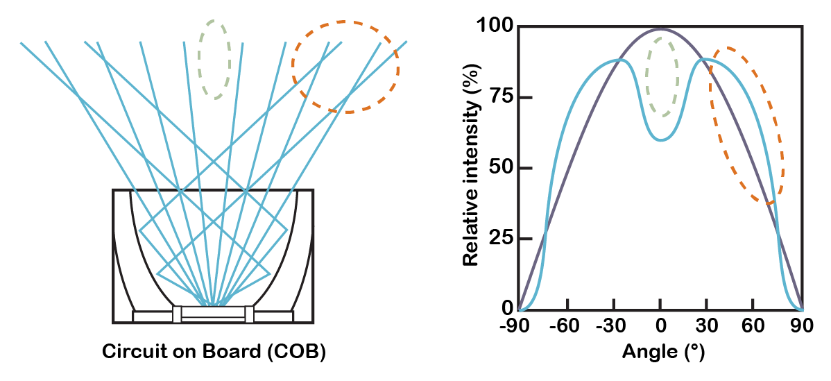
The curve will also be affected by the shape and volume of the encapsulation. Some LED suppliers provide photometric files in addition to FWHM plots for their LEDs. Of course at the hobbyists level just finding datasheets is challenging so it’s usually easier to just take some photos of the LED against a dark grey card.
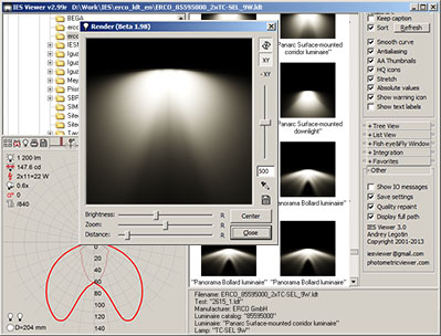
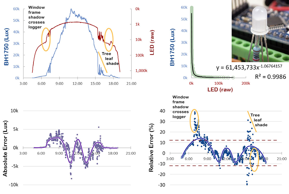
I could not find any information for the cheap eBay parts I’m using, so I decided to start with a 5050 LED with very little lens material over the LED:

The 5050 response crosses the Lambertian curve several times but the pattern still broadly follows the reflector cup diagram: the LED response shows a noon-time ‘deficit’ relative to the brighter ‘shoulders’ at midmorning & midafternoon.
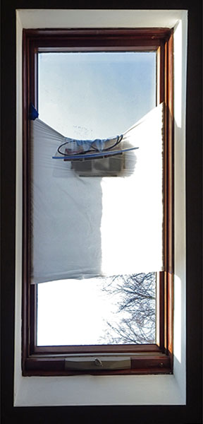
The logger was suspended in a south facing skylight window during these tests. Window frame shadow crossing events produce error spikes in opposite directions at ~6:30 am & pm, while wind-driven tree leaf shadows can produce errors in both directions from about 3:00 to 6:65 pm depending on whether the BH1750 or the LED is temporarily shaded. This was the least compromised location I could find in my urban environment.
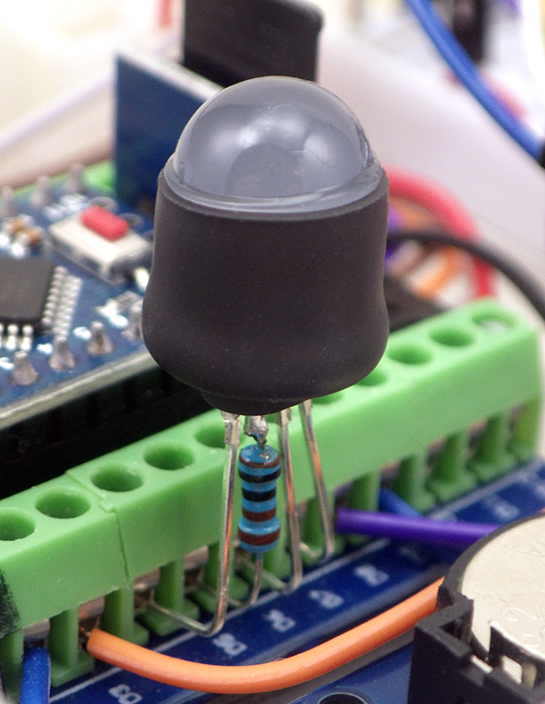
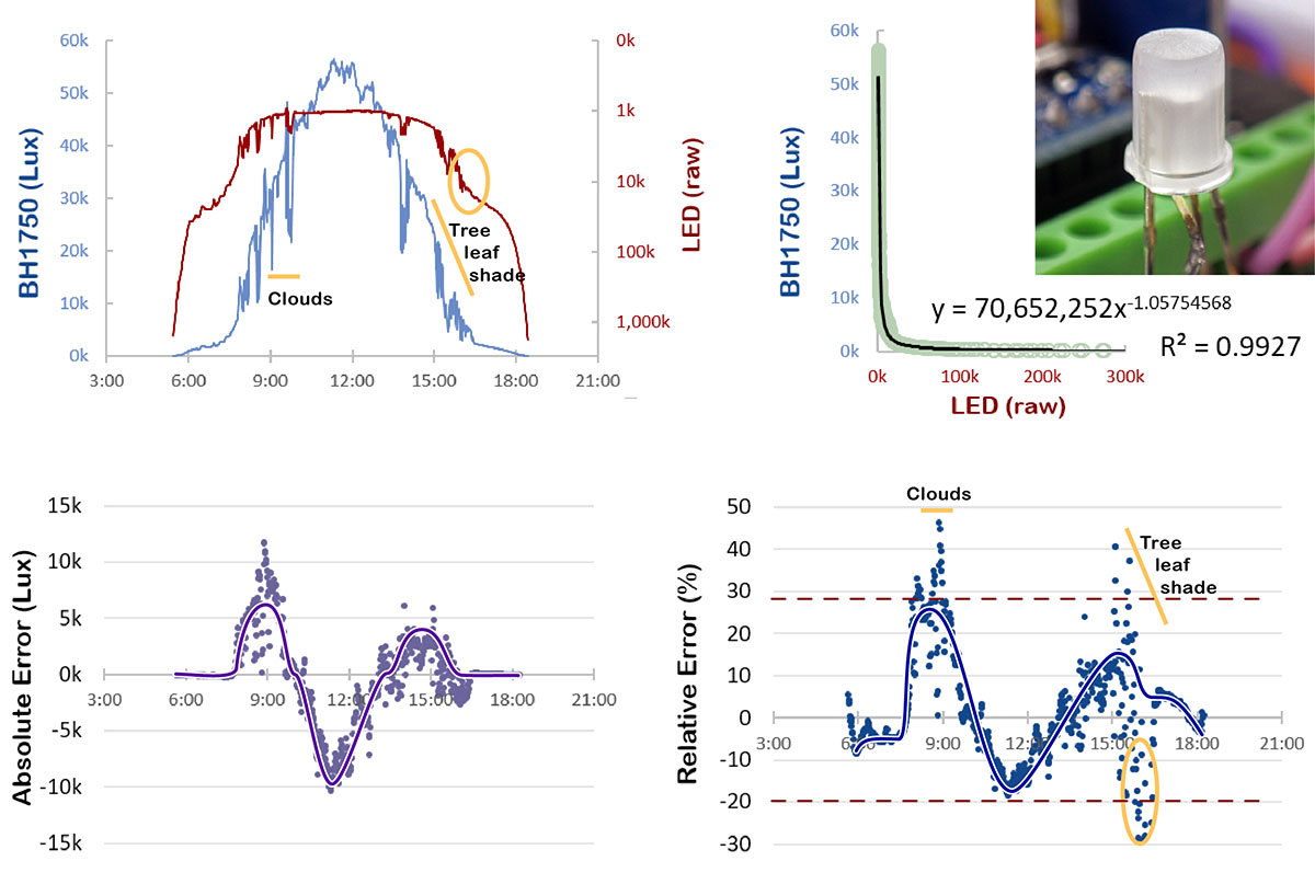
Now lets look at a clear 5mm RGB led:
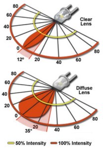
This non-diffused pattern is predicted by Figure 10 in the Broadcom datasheet, with the tight dispersion angle of lens producing a strong central ‘hot spot’. The overall pattern is inverted relative to the 5050 (which is primarily just the metal reflector cup) although the effect of the lens is much stronger. Adding small glass particles to the epoxy will diffuse the light, reducing the ‘focusing power’ of that lens:
The diffused 5mm response could be seen as an ‘intermediate mix’ of the 5050 & CLEAR led response curves. We can modify the response by sanding the top of the LED flat:
Removing the lens returns to a pattern similar to the 5050 – dominated by the effect of the metal reflector. So the key to making this calibration work will be finding a combination of lens & diffuser that brings the LED response closer to the BH1750:

PTFE tape is such a good diffusing material that it has disrupted the smooth refraction surface of the lens – essentially returning us to the 5050 pattern we saw with the physical removal of the lens from the 5mm led.

Finally we have a combination where the errors no longer show a clearly defined structure, with noise randomly distributed around zero. We still have ±10% cloud-noise but that is related to the time delta between the reference readings and the LED reading – so data from the LED alone will be cleaner. This two step modification will turn a garden variety LED into a reasonable ambient light sensor and the PTFE tape is thin enough that the LED is still useable as a status indicator.
Why is the LED a power law sensor?
Power laws are common in nature, arising when a relationship is controlled by surface area to volume ratios. As near as I understand it; when absorbed photons generate electron-hole pairs in the diode, only those pairs generated in the depletion region, or very close to it, have a chance to contribute to the discharge current, because there is an electric field present to separate the two charge carriers. In a reverse biased p-n junction, the thickness of this depletion region is proportional to the square root of the bias voltage. So the volume of diode material that can ‘catch photons’ is proportional to the voltage we initially placed across the diode – but this voltage falls as each captured photon reduces the capacitive charge stored at ‘surfaces’ of the diode. So the active volume gets smaller but the surface area is left relatively unchanged. I’m sure the low level details are more complicated than that, and power law patterns arise in so many different systems that it might be something entirely different (?)
