Category Archives: * Developing NEW sensors *

I’m developing a family of environmental monitors for use in caves and underwater, but the basic three component logger platform will support a wide range of different sensors.

Using the Nokia 5110 LCD with an Arduino Data Logger

Here I’ve added a the 5110 LCD to a logger recording data from a BME280 & Tipping Bucket Rain gauge. If the BME  survives in our field environment, this will become a standard configuration for our climate stations. I’m not holding my breath though, as we’ve tested half a dozen RH sensors so far and none of them have gone the distance in high humidity environments that occasionally go condensing.

This year I want to tackle some projects that need live data out, so I’ve been sifting through the many display options available for Arduino. Unlike flashier projects, my goal was to find one that I could add to existing logger builds without sacrificing too much of the multi-year lifespan I had worked so hard to achieve. The low power winner by a fair margin was the Nokia 5110 Liquid-crystal Display  which you can pick up for around $2 from the usual sources. With the back-light off these displays pull between 100-400 μA, depending on the number of pixels turned on.

This screen uses a PCD8544 controller and the SPI protocol.  It will tolerate 5V, but it works best at 3.3V, which is perfect when you are driving it from an 8mhz ProMini. Each pixel on the display is represented by a single bit in the PCD8544’s RAM. Each byte in RAM correlates to a vertical column of 8 pixels. The X coordinate works on a per-pixel basis, and accepts values between 0 and 83. The Y coordinate accepts values of 0 – 5 which on this 48 pixel high screen, corresponds to 6 “rows of bytes” in the controller’s RAM. So bitmaps can only be displayed on a per row (& column) basis. The display is quite sluggish compared to competitors like the 0.96 I2C monochrome OLED and you have to handle any processing overhead on the Arduino.

Most hookup guides assume that you can spare six control lines to run the display, which is not the case when your logger already has three indicator LEDs, I2c devices, one wire sensors and a couple of voltage dividers on the go.  However if you are willing to add a few resistors and occasionally toggle the power, you can bring that down to three wires and a power pin.

So many libraries, so little optimization…

This screen’s been around for a very long time, so there’s are a huge number of easy to use, highly functional libraries for Arduino. But they tend to focus on things like speed or endless font options which are not important for most data logging applications. And these libs assume your project can afford to lose up to ⅓ of the available program & variable memory just driving the display. Most also require the hardware SPI lines, but our project needs those for SD cards, which are finicky enough without some pokey LCD gumming up the works: the 5110 maxes out at 4mbps, and this slows the bus significantly .

Those fat libs were non-starters for our project, and I had almost given up on this display when I found Ilett’s Ardutorial offering a bare-bones method more suitable for our resource limited data loggers. If you haven’t discovered Julians YouTube channel yet then you are in for a treat because if Andreas Spiess is the maker worlds answer to Werner Herzog, then Julian is surely their equivalent to Bob Ross.  I don’t know if he’s growing “Happy little trees” with his DIY hydroponics, but I can say that the gentle timbre of his “Gooood morning all” reduces stress faster than a warm cup of Tea.  And his “Arduino sandwiches” are brilliant examples of minimalist build technique.

Driving the Nokia 5110 with shiftout

Everything I’m presenting here builds on his tutorials, so grab a mug and give ’em a watch:

Tutorial #1 – Connecting and Initial Programming
Tutorial #2 – Getting Text on the Display
Tutorial #3 – Live Numerical Data

This software SPI method (originally from arduino.cc?) requires no library at all, and shiftout commands work with any combination of digital pins; saving those hardware SPI lines for more important jobs.

Initial setup is explained in video #1 using two functions

void LcdInit(void)
{
digitalWrite(RST, LOW);            // not needed with pin powering!
digitalWrite(RST, HIGH);           // see below for details
LcdWriteCmd(0x21);                 // extended commands 
LcdWriteCmd(0xB8);                 // set Vop(contrast) // you may need to tweak
LcdWriteCmd(0x04);                 // set temp coefficient 
LcdWriteCmd(0x14);                 // bias mode 1:40 // you may need to tweak this
LcdWriteCmd(0x20);                 // basic commands 
LcdWriteCmd(0x0C);                 // normal video
for(int i=0; i<504; i++) LcdWriteData(0x00);  // clear the sceen
} 
void LcdWriteCmd(byte cmd)
{
digitalWrite(DCmodeSelect, LOW);    // low for commands, high for data 
digitalWrite(ChipEnable, LOW);      // not need with pin-power
shiftOut(DataIN, SerialCLK, MSBFIRST, cmd);  // transmit serial data 
digitalWrite(ChipEnable, HIGH);     // not need with pin-power
} 

After that you need is a function to position the cursor and a font stored in a byte array (in this example called ASCII[][5])

void LcdXY(int x, int y)
{
LcdWriteCmd(0x80 | x);              // Column
LcdWriteCmd(0x40 | y);              // Row  
} 

Then three short cascading functions let you send a string of ascii characters to the display:

void LcdWriteString(char *characters)
{
while(*characters) LcdWriteCharacter(*characters++);
} 
void LcdWriteCharacter(char character)
{
for(int i=0; i<5; i++){
LcdWriteData(pgm_read_byte(&ASCII[character - 0x20][i])); 
}
LcdWriteData(0x00);            //one row of spacer pixels between characters
} 
void LcdWriteData(byte dat)
{
digitalWrite(DCmodeSelect, HIGH);    // High for data 
digitalWrite(ChipEnable, LOW);  
shiftOut(DataIN, SerialCLK, MSBFIRST, dat);  // transmit serial data 
digitalWrite(ChipEnable, HIGH);
} 

Julians original implementation included a 500 byte 5×7 font.h file (which you can find at several locations) and  I’ve rolled that font array into some code based on his work and posted it to the Cave Pearl Project’s repo .  You will find lots of other examples based on the shiftout method on Github, but for some reason many people insist in retooling that tiny bit of code into, you guessed it, even more libraries

You’ll also find plenty of other drop-in font definitions with Google, but for small 5×7’s, it doesn’t take that long to roll your own by clicking the boxes in an online font creator. and then copying the byte pattern into a bin-hex converter. This also gives you the option of creating custom icons by using a non-standard bitmap for some of the less frequently used ascii characters. Keep in mind that you don’t need to store the entire alphabet if you are only sending a few letters to the screen (like ‘T+P’ or ‘RH%’, etc …) extracting only the letters you need to a reduced font array could save a lot of memory.

So your reduced font array could look something like this:

const byte ASCII[][5] =
{
{0x7f, 0x09, 0x19, 0x29, 0x46}  // 52 R
,{0x7f, 0x08, 0x08, 0x08, 0x7f} // 48 H
,{0x23, 0x13, 0x08, 0x64, 0x62} // 25 %
,{0x01, 0x01, 0x7f, 0x01, 0x01} // 54 T
,{0x08, 0x08, 0x3e, 0x08, 0x08} // 2b +
,{0x7f, 0x09, 0x09, 0x09, 0x06} // 50 P 
};  

If you do that you’ll need to send text to the screen character-by-character because the ASCII based [character – 0x20] calculation won’t work any more.

I tweaked Julians code in a couple of important ways. First, I added PROGMEM to move the font(s) into the program memory space. Second, I added a method to print large numbers to the screen by repeating the same WriteString->WriteCharacter->WriteData pattern two times: once for the “upper half” of the numbers, and then again for the “lower half” of the numbers after re-positioning the cursor to the next line.

To make this limited large-number font I first composed a black & white bitmap for each number with a graphic editor, and then loaded that .bmp file into the LCD assistant program as described in this instructables tutorial.  I started with a bitmap that was 11 pixels wide, by 16 pixels high (though you can use any arbitrary size you want – just remember to leave the blank spacer row at the bottom) and for this two-pass ‘sliced-letters’ method I set vertical & little endian encoding in LCD assistant. I then put the top 11 bytes in the Big11x16numberTops[] array & the lower 11 bytes for each number in the Big11x16numberBottoms[] array.

It takes two passes to print each large number to the screen:

LcdXY (0,2);              //top half of the double-size numbers
LcdWriteBigStringTops(dtostrf(voltage,5,2,string));  
LcdXY (0,3);              //bottom half of the numbers 
LcdWriteBigStringBottoms(dtostrf(voltage,5,2,string));

And some slightly modified functions that refer to the corresponding number-font array:

void LcdWriteBigStringTops(char *characters)
{
while(*characters) LcdWriteBigCharacterTops(*characters++); 
} 
void LcdLcdWriteBigCharacterTops(char character)
{
for(int i=0; i<11; i++){
if((character - 0x2d)>=0){
LcdWriteData(pgm_read_byte(&Big11x16numberTops[character - 0x2d][i]));
}
}
LcdWriteData(0x00);  //one row of spacer pixels inserted between characters  
} 

Those number printing functions could be eliminated with better use of pointers, but I liked having the readability afforded by a few extra lines of code.

Reducing the number of control lines

The stuff I posted on Github assumes you are using a standard 6-pin arrangement shown in most Nokia 5110 hookup guides you will find on the web. But once I had that wrangled, I realized that it would be possible to reduce the number pins needed to drive the display.  You will have to tweak that default example by commenting out the RS & CS commands if you implement the pin-power changes I’m suggesting here… 

I use Deans micro-plugs  for multi-wire applications like this. The unused pin here is the normal Vcc, with the A0 pin-power supply indicated with a dash on the red line.

The shiftout method can be used with any pins you want, and most of my builds have A0-A3 available. With those dedicated wires the PCD8544’s chip select (CS) line can be connected to GND telling the screen that it’s always the selected device. This would be bad if it was connected to the hardware SPI lines shared with the SD card, but since we are using re-purposed anlaog lines, there is no conflict. One minor drawback is that since we are now using all the analog lines (I use A6 & A7 too) we can’t read a floating pin for RandomSeed().

Getting rid of the RESET line is a little trickier. The data sheet says that the RS line must be low while power stabilizes and should then be pulled high within 100ms of power on. Several people create an auto-reset situation by connecting the screens reset to the Arduino’s reset line. Others make the low-high transition with an RC network across the supply for a delayed rising signal. This can even be driven by the DC line (which is low in command mode and high in data mode) 

But I had something else in mind, since I wanted to power the entire display from a digital pin because the power draw with the display off is still about 70uA. This accumulates into a significant amount of wasted power over a multi-year deployment.

Reducing Back-light Current

OR … a photocell divider embedded in that clear epoxy would let you enable the backlight dynamically – with the appropriate mosfet for the connection type.

If you use the back-light in the default configuration, the screen can potentially draw up to 80mA (4 white LEDs at 20mA each). The back-light pin is usually connected to a transistor, so you can PWM all 4 LEDs at once for variable lighting control, but the peak currents are still too high for direct pin-powering unless you add some kind of series resistor.  A 10k pot gives you a simpler method to adjust the screen brightness, but I found that a 3k3 series resistor brought the total display current down to ~1mA with decent readability ( & blue LEDs are brighter than white).  Adding an in-line slide switch provides a way to completely disable the back-light for long deployments.  With the entire display safely below Arduino’s pin-current limit, you can then power it by writing a driver pin high or low in output mode.

#define n5110PowerPin  A0          // power the 5110 screen from pin A0 (RED)
#define n5110modeSelect A1         // 6.1.9 D/C: mode select (BLUE)
#define n5110SData A2              // 6.1.7 SDIN: serial data line (WHITE) 
#define n5110SCLK A3 ;             // 6.1.8 SCLK: serial clock line (YELLOW)
// lines not needed any more: 
// #define n5110RST  Now -> 4.7k to power A0
// #define n5110ChipEnable  Now -> GND

This gives you a way to perform a hard reset any time you want provided you tie the screens RS line to that switched power with a 4k7 pullup resistor, and re-run the initialization sequence after restoring power.

Boards with pin vias on both sides make it easier to add the RST & CE connections. The orange wires shown here thread through the housing to a slide switch which disables the backlight connection for surface deployments. This example connects power to the backlight, but with other screens you might have to connect BACKLIGHT to GND.

Enabling the screen now looks like this in setup:

pinMode(n5110PowerPin, OUTPUT);
digitalWrite(n5110PowerPin, HIGH);
pinMode(n5110modeSelect, OUTPUT);
pinMode(n5110SData, OUTPUT);
pinMode(n5110SCLK, OUTPUT); 
LcdInit(); // shiftout takes control of Mode, Data & SCLK lines at this point

To turn off the screen you pull all the control lines low:

digitalWrite(n5110PowerPin, LOW);        
digitalWrite(n5110modeSelect, LOW);                
digitalWrite(n5110SData, LOW);                
digitalWrite(n5110SCLK, LOW);                         

All four control lines must be brought low when you de-power the display or you will get a 13mA leak current through the controller after vcc goes low. Only the power pin needs to be driven high to start the screen later in the main loop, but don’t forget to run the init each time you power up.

My tests so far have shown reliable operation of pin-powered 5110’s through more than 8000 ‘long-sleep’ power cycles. In applications where I want to display data on the screen on for long periods of time,  I still depower the screen during the new sensor readings. This lets me know when the logger is capturing data and forces a periodic re-synch with the bus. I don’t know how long these displays would run continuously without that step, but I’m sure the coms would eventually go AWOL without some kind of regular reset.

Potting the Nokia 5110 display

Contraction of the epoxy created pressure burns on the LCD when I did a single large pour to pot the screen.

No screen is much use on our project unless it can withstand some bumping around in the real world, and ideally we want one that is dive-able. For several years my go-to solution has been to pot surface mounted LED’s and sensors in Loctite E30CL. I like this epoxy because the slow cure usually sets clear because bubbles have time to rise to the surface without a vacuum treatment. My first attempts looked great the night of the pour, but I got a nasty surprise the following morning. You see I usually mount sensors in small ½-1 inch wells, but the 5110 required a ring more than 2” in diameter. The contraction of the epoxy in this 10mm deep well caused pressure marks on the edges of the screen, and a significant brown spot in the center of the display where the text became inverted.

Successive small pours worked better. Here the back-light reflects off of the edges of the epoxy that seeped under the screen before it finished setting. The display in this photo has a 3k3 series resistor in the backlight circuit.

The next attempt was much more successful, as I built up the epoxy a few mm at a time like the layers of an onion. As each layer hardened, it protected the screen from the contraction of the subsequent layers above.  The trick was to bring the first pour to the base of the pcb, and the second pour to “just barely” cover the surface of the screen. The epoxy penetrates about 1/3 of the way into the display housing but this does not interfere with readability as those edges are invisible under natural lighting conditions. That epoxy is actually under the LCD, in the air gap between the transparent glass LCD sandwich and the white reflector plastic which holds the thin LCD in place between the metal rim and the PCB.  I’ll try future pours at different angles to see if that lets the space under the LCD fill completely. Looking at the epoxy penetration, it’s clear that the black edges in pour #1 were places where the LCD was compressed on both sides, and the brown discoloration was from pressure on top with no support below. 

Seawater caused severe fogging of the potting epoxy after only three days in service. Originally a concession to my aging eyes, the large fonts really saved our bacon when this reaction occurred.

The results for the second batch looked good and the screens worked beautifully with full marine submersion for about two days. Then some kind of chemical reaction with the sea-water started fogging the epoxy, and by day three I was glad I’d created the large number fonts because the 5×7’s were completely unreadable.   Once we were back home, a bit of elbow grease & 800 grit removed the foggy surface rind, and a layer of conformal coating restored clarity. I think my next builds will add the coating to the epoxy surface at the start.

I also noted some screen discoloration from pressure at about 3m depth, indicating that even a thick layer of epoxy bows too much for a deeper deployment. I’ve ordered some 1/4“ plexiglass disks to provide a surface with a bit more chemical resistance, and will post an update on how that works after the next fieldwork trip. I’m hoping that provides a bit more pressure protection too, but the shore hardness of the epoxy is 85, and PMMA (plexiglass) is only a few steps above that at 90. I might try polycarbonate as well.

Other Fun stuff:

There is so much more to explore with this screen, including live graphing libraries, and display controls so I expect it will keep me amused for a while since I can add it to any of the current logger builds. Several are out in the wild now for long term tests, and I’m currently working on a script to move those fonts (and a few other things) into the 328p’s internal eeprom. If all goes well I’ll release that ultra low memory footprint version of the code shortly. 

Cheers for now.

Addendum 2018-08-24

After several builds using the this LCD screen I finally got around to storing those font arrays in the Arduino’s internal EEprom. Works a treat, and frees a good chunk of PROGMEM space with very little change to the core functions. With fonts in EEprom, the remaining Nokia 5110 functions compile to a little over 400 bytes of program storage and 10 bytes of dynamic. (not counting EEprom.h) And that’s with three copies of the output functions because of the simple 2-pass method I’m using to display the large numbers.  A small price to pay for live data output on our loggers!

Addendum 2018-10-17

Because of that pressure problem with the 5110 I decided to try out the 0.96″ OLED screens which sell for about $3 on eBay.  When the first batch arrived I was pleasantly surprised by how well they stood up to pressure on their surface. Then I found the SPI version of the SSD1306 OLED can be driven by essentially the same code as the PCD8544 (with the exception of the init & XY functions which are specific to each controller).

Adding the SSD1306 OLED Screen to an Arduino Logger (without a library)

I’m connecting the OLED with the same analog line connections used for the Nokia, but I’ve added a delayed-high RC bridge because the OLED is pickier about the reset input than the Nokias. In hindsight a similar method is probably a good idea for the Nokia screens as well, though you might need to experiment a bit with the resistor/cap values to get the timing right.

Addendum 2020-11-15:

Two I2C 0.96″ OLED displays make a highly useful addition to the basic three module logger

I finally got around to adapting this  eeprom/fonts method for use with I2C displays:

Adding two OLED displays to your Arduino logger

Tutorial: How to Configure I²C Sensors with Arduino Code

I’ve spent the last year in the ‘uncanny valley’ of the Arduino. That’s the point where you understand the tutorials at Arduino.cc, but still don’t get much from the material on gitHub because trained programmers would never stoop to using the wire.h library when they could just roll their own in native C++ using the avr-g compiler.  The problem with establishing sensor communication at the level of the TWI peripheral inside the AVR is that there are so many fiddling details to keep track of that it quickly overruns the 7±2 things this average human can hold in his head at one time: Computers aren’t the only things that crash after a buffer overflow!  So this post is meant to be a chunking exercise for beginner-intermediate level people who want to get a new sensor working using the standard IDE.  I’ve tried to distill it all down to things that I run into frequently, but there’s still a lot of material here:  So pour yourself a cuppa before diving in...

The great strength of I2C is that you can put so many sensors on the same four wires. But for units with several pre-made modules connected you might have to remove a few smd resistors from the breakouts, or the pull-up on the bus might become too aggressive. Most of the time I just leave them on, so I can extend the wire length, or crank up the bus clock

REGISTERS are simply memory locations inside an I²C device. The summary of how many registers there are in a given sensor, and what they control or contain is called a register map. Most of the information on the sensor’s datasheet is about explaining how each register functions, and they can be quite a slog to read through because the information is rarely presented in an intuitive way.

To give you a sense of what I mean by that: take a look at page 14 of the manufacturers datasheet for the ADXL345 accelerometer:

A document only a hardware engineer could love…

Then take a look at the interactive register map for that sensor over at the i2cdevlib site:

Even if you’ve never worked with registers before, jrowberg’s visual grid layout makes it easy to see how the sensor’s memory is divided into sections, which are doing different things.

There are many kinds of registers but for this introduction I am going to group them into three general types: Control, Data and Status registers, and provide brief examples of code that you can use to work with each of them. The functions named with the i2c_ prefix should be generic enough to work with most I²C sensors, but I’ll also be referring to a few specific cases to show how you might need to modify those basic functions.

1) Control Registers

Most sensors change how they operate based on the values stored in control registers. Think of control registers as banks of On/Off switches, which you turn on by setting a bit to 1 and turn off by setting that bit to 0.  I²C chip-based sensors often have a dozen or more operational settings for things like bit-depth, sampling speed, noise reduction, etc., so you usually need to set bits in several different control registers before you can actually take a reading. And sometimes there are “special chip functions” that perform some kind of post processing on those sensor readings that would be hard to replicate on the Arduino. These can add an extra layer of control settings to take care of when you initialize the sensor.

Arduino’s wire library can only transfer 8-bit bytes over the I²C bus, so that’s the smallest amount of information you can write into a register memory location at one time. This can potentially change eight of those control switches simultaneously and, for parameters that are controlled by more than one bit, sometimes it’s actually required that you set them in one register-writing operation.  Most people use byte variables for the sensor’s bus and register memory addresses, but once you’ve figured out the pattern you need to set up in control register switch-bits, it helps to write that information as a long form binary number (eg. 0b00001111) so you can see the on/off states when you read through your code. 

Writing a byte to a sensor’s control register can be done with four basic steps:

Wire.beginTransmission(deviceAddress);  // Attention sensor @ deviceAddress!
Wire.write(registerAddress);   // command byte to target the register location
Wire.write(dataByte);                           // new data to put into that memory register
Wire.endTransmission();

The I²C deviceAddress is set by the manufacturer but some can be modified from their defaults by connecting solder pads on the breakout board.  Since the bus address of a given sensor IC can vary from one module to the next I keep Rob Tillaart’s bus scanner handy to find them, and more importantly to discover when two sensors are fighting with each other by trying to use the same address on the bus.  The registerAddress moves a pointer inside the chip to the memory location you specified. You can think of this pointer as a read/write head and once that pointer is aiming at a specific register, the next byte you send along the wires will over-write the data that was previously stored there.

The startup default values for a given control register are often a string of zeros because all the chip functions being controlled by that register are turned off. Unfortunately this means you’ll find lots of poorly commented code examples out there where people simply write zero into a control register without explaining which of the eight different functions they were aiming for because seven of those were still at their default zero-values anyway.

Reading data from a sensors memory register(s) requires two phases:

Wire.beginTransmission(deviceAddress);    // get the sensors attention 
Wire.write(registerAddress);    // move your memory pointer to registerAddress
Wire.endTransmission();           // completes the ‘move memory pointer’ transaction

Wire.requestFrom(deviceAddress, 2); // send me the data from 2 registers
firstRegisterByte = Wire.read();             // byte from registerAddress
secondRegisterByte = Wire.read();       // byte from registerAddress +1

The first phase tells the I²C slave device which memory register that we want to read but we have complete the read operation in two separate steps because the wire library buffers everything behind the scenes and does not actually send anything until it gets the Wire.endTransmission(); command.  The second phase is the data reading process and you can request as many bytes as you want with the second parameter in Wire.requestFrom .  The memory location pointer inside the sensor increments forward automatically from the initial memory register address for each new byte that it sends. (The ‘dummy-write 1st’ method is similar to the  procedure you’d use when doing a random data read from larger eeprom memory chips as well as sensors)

These simple patterns are at the heart of every I²C transaction, and since they are used so frequently, they often get bundled into their own functions:


byte i2c_readRegisterByte (uint8_t deviceAddress, uint8_t registerAddress{
byte registerData;
Wire.beginTransmission(deviceAddress);              // set sensor target
Wire.write(registerAddress);                                     // set memory pointer
Wire.endTransmission();
// delete this comment – it was only needed for blog layout.   
Wire.requestFrom( deviceAddress,  1);     // request one byte
resisterData = Wire.read(); 
// you could add more data reads here if you request more than one byte
return registerData;           // the returned byte from this function is the content from registerAddress
}
// delete this comment – it was only needed to maintain blog layout
byte i2c_writeRegisterByte (uint8_t deviceAddress, uint8_t registerAddress, uint8_t newRegisterByte
 {
byte result;
Wire.beginTransmission(deviceAddress);
Wire.write(registerAddress);  
Wire.write(newRegisterByte); 
result = Wire.endTransmission(); // Wire.endTransmission(); returns 0 if write operation was successful
// delete this comment – it was only needed for blog layout.
//delay(5);  // optional:  some sensors need time to write the new data, but most do not. Check Datasheet.
if(result > 0)  
{ Serial.print(F(“FAIL in I2C register write! Error code: “));Serial.println(result); }
// delete this comment – it was only needed for blog layout. 
return result;    // the returned value from this function could be tested as shown above
//it’s a good idea to check the return from Wire.endTransmission() the first time you write to a sensor 
//if the first test is okay (result is 0), then I2C sensor coms are working and you don’t have to do extra tests

//NOTE: copy/pasting code from blogs/web pages is almost guaranteed to give you stray/302 errors because
//of hidden shift-space characters that layout editors insert. Look at the line your compiler identifies as
//faulty, delete all the spaces and/or retype it slowly and carefully ensuring you enter only ASCII characters.


Those two functions will let you control the majority of the I²C sensors on the market, provided you can figure out the correct pattern of bits to send from the datasheet. A common strategy for keeping track of the multi-bit combinations that you want to load into your sensor control registers is to declare them with #define statements at the beginning of your program, which replace the human readable labels with the actual binary numbers at compile time.

For example the ADXL345 can range from 3 samples per second to 1600 samples per second, depending on four bits in the ADXL345_BW_RATE register. A set of define statements to represent those bit combinations might look like:

byte ADXL345_Address=0x53;     // the sensors i2c bus address (as a hex number)
byte ADXL345_BW_RATE=0x2c;    // the memory register address
#define ADXL345_BW_1600  0b00001111
#define ADXL345_BW_800    0b00001110
#define ADXL345_BW_400    0b00001101
#define ADXL345_BW_200    0b00001100
#define ADXL345_BW_100    0b00001011
#define ADXL345_BW_50      0b00001010
#define ADXL345_BW_25      0b00001001
#define ADXL345_BW_12      0b00001000
#define ADXL345_BW_6        0b00000111
#define ADXL345_BW_3        0b00000110
etc…. Note that all of these combinations assume normal power mode (bit4=0)

So a command to set the sampling rate to 50 Hz could be written as:

i2c_writeRegisterByte(ADXL345_Address, ADXL345_BW_RATE, ADXL345_BW_50);

 The cool thing about using defines is that they do not use any ram memory like byte variables would. And you can usually find code examples on gitHub where someone has transcribed the entire register address list into a set of defines, which you can simply copy and paste into your own code. This saves you a great deal of time, though there’s always the chance they made a transcription error somewhere. Also note that typical datasheets & ‘c’ language examples express those numbers as hex “0x0F” instead of “0b00001111” and you can leave them in that format if you wish.

Writing a whole byte to a register is pretty straightforward, but it gets more complicated when you need to change only one of the bit-switches inside a control register. Then the standard approach is to first read out the register’s current settings, do some bit-math on that byte to affect only bit(s) you want to change, and then write that altered byte back into register’s memory location.

But bit-math syntax is one of those “devils in the details” that makes relatively simple code unreadable by beginners. The bit operators you absolutely must be familiar with to understand sensor scripts you find on the web are: the bitwise OR operator [|] , the bitwise AND operator [&], the left shift [<<] and the right shift [>>] operators.  Fortunately there is an excellent explanation of how they work over at the Arduino playground, with a set of bit-math recipes in the quick reference section that let you reach into a byte of data and affect one bit at a time.  Be sure to parenthesize everything when using bitwise operators because the order of operations can be counter-intuitive, and don’t worry if you have to look up the combinations every time because most people forget those details once they have their code working. I know I do. 

Two particularly useful procedures:

x &= ~(1 << n);   // AND inverse (~) forces nth bit of x to be 0. All other bits left alone
x |= (1 << n);       // OR forces nth bit of x to be 1.  All other bits left alone

And these let us add a third function to the standard set which will turn on or turn off one single bit switch in a sensors control register:

byte i2c_setRegisterBit ( uint8_t deviceAddress,  uint8_t registerAddress,  uint8_t bitPosition, bool state )  { 
 byte registerByte, result;
registerByte = i2c_readRegisterByte ( deviceAddress,  registerAddress ); // load the current register byte
// delete this comment – it was only needed to maintain blog layout
if (state) {   // when state = 1
  registerByte |= (1 << bitPosition);   //bitPosition of registerByte now = 1
//or use bitSet(registerByte, bitPosition); 
  }  
else {           // when state = 0
   registerByte &= ~(1 << bitPosition);   // bitPosition now = 0
//or use bitClear(registerByte, bitPosition); 
  }
// now we load that altered byte back into the register we got it from:
result = i2c_writeRegisterByte ( deviceAddress,  registerAddress,  registerByte );
return result;   // result =0 if the byte was successfully written to the register


The ADXL345 accelerometer supports low power modes that use about 1/3 less power than the ‘standard’ operating modes.  The sensor is not turned off, but the bandwidth is reduced somewhat, so the sensor responds more slowly to things like tap inputs.
An example which sets the single bit enabling this low power mode might look like:

i2c_setRegisterBit( ADXL345_ADDRESS,  ADXL345_BW_RATE,  5,  );

Many I2C sensors have power saving features like that which rarely get utilized. Note that bit position numbering starts with 0 and counts from the left OR the right hand side depending on the sensor manufacturer. 

Some devices have control registers that are 16-bits wide. These get treated as a pair of 8-bit bytes that are read-from or written-to sequentially. You only have to specify the device & register address once at the beginning of the process because the sensors internal memory pointers get incremented automatically during the process.

This adds an extra wire.write step to the basic register writing operation:

Wire.beginTransmission(deviceAddress);
Wire.write(registerAddress);
Wire.write(MSB_registerData);    // Send the “upper” or most significant bits
Wire.write(LSB_registerData);     // Send the “lower” or least significant bits
Wire.endTransmission();

The MCP9808 is a common temperature sensor that uses 16-bit control registers.  Setting “bit 8” of the CONFIG register to 1 puts the sensor into shut down mode between readings and setting that bit to 0 starts the sensor up again. (yes, that’s opposite to the usual on/off pattern…)  The 8-bit limitation of the I²C bus forces us to retrieve the register in two separate bytes, so bit 8 of the 16 bits described in the datasheet ends up in the zero bit position of MSB. 

A custom function shutting down the MCP9808 might look like this:  

#define MCP9808_i2cAddress          0x18    // defines in setup are an alternative to using variables
#define MCP9808_REG_CONFIG   0x01    // the compiler swaps the text-name for the # at compile time
// delete this comment – it was only needed to maintain blog layout
void mcp9808shutdown()      //since we used defines, we did not pass any byte variables into the function

 byte MSB, LSB;
 Wire.beginTransmission(MCP9808_i2cAddress);
 Wire.write(MCP9808_REG_CONFIG);
 Wire.endTransmission();
// delete this comment – it was only needed to maintain blog layout
 Wire.requestFrom(MCP9808_i2cAddress, 2); //request the two bytes
 MSB = Wire.read();       // upper 8 bits described in data sheet as 15-8
 LSB = Wire.read();        // lower 8 bits described as 7-0 in the datasheet
// delete this comment – it was only needed to maintain blog layout
 MSB |= (1 << 0); // bitmath forces MSB bit0 (which is ‘bit8’ in the datasheet) to value one
 // using MSB &= ~(1 << 0); here would start the sensor up again by forcing the bit to zero
// delete this comment – it was only needed to maintain blog layout
 Wire.beginTransmission(MCP9808_I2cAddress);  // now write those bytes back into the register
 Wire.write(MCP9808_REG_CONFIG);
 Wire.write(MSB);                          // the one we modified
 Wire.write(LSB);                           // unchanged
 Wire.endTransmission();
}


This ‘position x becomes position y’ translation is common stumbling block for beginners working with multi-byte registers – especially when you add reverse order position numbering into the mix.  But there’s another gotcha with 
control registers that’s even more frustrating if you don’t catch it on your first pass through the datasheet:  Sometimes there are special “write protection” registers that have to be set before you can change any of the other control registers, and these have to be changed back to their “protecting” state before those new settings take effect. You might not get any error messages, but nothing will work the way it should until you get the protection bits disabled and re-enabled in the right sequence. Fortunately less than 20% of the sensors I’ve worked with have this  feature.

Another thing to watch out for are old code examples on the web that appear to be using integer variables to store device and memory register locations, with statements like Wire.send((int)(eepromaddress >> 8));  The I²C wire library only sends bytes/uint8_ts, but people got away with this (int) cast  because it was being corrected behind the scenes by the library, which re-cast the value into a byte at compile time.  The (byte) data type on Arduino is interchangeable with the (uint8_t) variables you see in most C++ coding tutorials. 

2) Data registers

Unlike a control registers bank-of-switches, I think of data output registers as containers holding numbers which just happen to be stored in binary form. Since eight bits can only hold decimal system values from 0 to 255 you usually have to “re-assemble” larger sensor output values from bytes stored in consecutive memory locations. For sensors like the ADXL345 you can concatenate the two 8-bit bytes into one 16-bit integer variable by shifting the MSB left by 8 positions and merging in the LSB with a bitwise OR :

Wire.beginTransmission(deviceAddressByte);  // the pointer setting transaction
Wire.write(registerAddressByte);
Wire.endTransmission();

Wire.requestFrom(deviceAddressByte,2);       // request two bytes
LSB = Wire.read();                                                // byte from registerAddressByte
MSB = Wire.read();                                              // byte from registerAddressByte +1
int combined = (int)MSB;             // MSB now in rightmost 8 bits of combined int
combined = combined<<8;          // shift those bits to the left by 8 positions
combined |= LSB;     // logical OR keeps upper bits intact and fills in rightmost 8 bits

Those steps are usually written in one single line as:

int combined = (((int)MSB) << 8) | LSB;

There are several other ways to combine bytes and some sensors send the MSB first – so you have to check the register map in the datasheet to know the order of the bytes that arrive from the output registers when you request multiple.

Now if you are thinking that looked too easy – you’re right! Most hobby market I2C sensors only have a 12-bit ADC, and since memory is a limited resource there are often status register bits mixed in with the data held in the MSB. Since these bits are not part of the sensor reading, you need to &-mask them away before you combine the MSB & LSB. It gets trickier when the sensor output can be a positive or a negative number because signed and unsigned integers are distinguished from each other by a special “sign” indicator bit, which can accidentally be turned into a “number” bit by bit shifting. (see: ‘sign extension’ in that bit math tutorial )

The temperature data output register in the MCP9808 is a good example of both of these issues:

Bits 15-13 (which become the top 3 bits of the upperByte in the code below) are status indicator flags identifying when high & low temp. alarm thresholds have been crossed. Bit 12 is a sign bit (0 for +ve temperature or 1 or -ve temps). The remaining bits 11-8 (=bits 3-0 of the upperByte) are the most significant 4-bits of the 12-bit integer representing the temperature.

So a sensor-specific approach to reading the temp. from an MCP9808 might look like this:

int TEMP_Raw;
float TEMP_degC; 

// spacer comment for blog layout
Wire.beginTransmission(0x18);    // with mcp9808 bus address written in hex
Wire.write(0x05);                             // and the temperature output register
Wire.endTransmission(); 
Wire.requestFrom(0x18, 2); 
byte UpperByte = Wire.read();          // and sometimes the MSB is called the “highByte” 
byte LowerByte = Wire.read();          // sometimes called the “lowByte” 
// spacer comment for blog layout
UpperByte = UpperByte & 0b00011111;  // Mask away the three flag bits
//easier to read when the mask is written in binary instead of hex
// spacer comment for blog layout
//now we use a mask in a slightly different way to check the value of the sign bit:
if ((UpperByte & 0b00010000) == 0b00010000)  {          // if sign bit =1 then temp < 0°C
UpperByte = UpperByte & 0b00001111;                             // mask away the SIGN bit
TEMP_Raw = (((int)UpperByte) << 8) | LowerByte;    // combine the MSB & LSB
TEMP_Raw-= 256;   // convert to negative value: note suggested datasheet calculation has an error!
 }
else  // temp > 0°C  then the sign bit = 0  – so no need to mask it away
 {
TEMP_Raw= (((int)UpperByte) << 8) | LowerByte;
 }
// spacer comment for blog layout
TEMP_degC =TEMP_Raw*0.0625;


Typically a data output register will continue to hold the last sensor reading until it is refilled with the next one. If your sensor takes a long time to generate this new reading (30-250 ms is typical, while some can take up to a second) and you read the registers before the new data is ready, you can end up loading the previous sensor reading by mistake. That’s where status registers come to the rescue.

3) Status registers

These tell you if if a specified type of event has occurred and I think of these registers as a set of YES/NO answers to eight different questions. The most commonly used status register is data ready [usually labeled DRDY] which sets a bit to 1=true when a new sensor reading is available to be read from the related output registers. Another common status register is one that becomes true if a sensor reading has passed some sort of threshold (like a low temperature alert, or a falling/tilt-angle warning).

A function to check the true=1/false=0 state of a single DRDY bit inside an 8-bit status register might look like this: 

bool i2c_getRegisterBit (uint8_t  deviceAddress, uint8_t  registerAddress, uint8_t  bitPosition) {     
byte registerByte;
registerByte = i2c_readRegisterByte(deviceAddress, registerAddress);
 return ((registerByte >> bitPosition) & 0b00000001);  // or use (bitRead(registerByte, bitPosition))
 }
// delete this comment – it was only needed to maintain blog layout
 //  You could use i2c_getRegisterBit to check the DRDY status bit with a do-while loop
//  and only move on to reading the sensor’s data output registers after the DRDY bit changes to 1
// delete this comment – it was only needed to maintain blog layout
bool dataReady=0;
do {
dataReady= i2c_getRegisterBit(deviceAddress, statusRegAddress, DRDYbitPosition);  
} while ( dataReady==0 );        // processor gets cycled back through this loop until DRDY=1


Holding the processor captive in a status-bit-reading loop is very easy to do, but it is usually avoided unless you are trying to capture a series of sensor readings quickly.  Most status register bits can be mapped to physical alarm output lines on the sensor module, and these can be used to trigger a hardware interrupt pin (D2 & D3) on the Arduino.  This lets you to setup an interrupt service routine (ISR) which grabs that new reading even faster than a bit reading loop. And since hardware interrupts can be used wake a sleeping processor, the interrupt method also lets you put your data logger to sleep until something actually happens. 

The only drawback to the ISR method is that the sequence of register settings you need to follow to create hardware alarms is another multi-step process to add to your sensor initialization code.  The conceptual pattern is usually something like:

  1. Disable the sensor’s global interrupt control bit (if there is one)
  2. Enable the sensors triggering function   (eg:  a max. temperature alert)
  3. Load register(s) with the parameter value for that trigger (eg:  52.5°C)
  4. Turn on the status register that listens to that triggering function
  5. Map that status register bit to a hardware output line
  6. Re-enable the global interrupt control bit

This LSM303 combined accelerometer / magnetometer sensor has two alarm outputs in addition to DRDY. So you could map the Accelerometers DRDY signal to int1, and the Magnetometers DRDY to DRDY.  Just to make life interesting with this sensor, the 3-axis output data  registers are arranged in a different order  on the magnetometer than  they are on the accleerometer. This is typical for multi-sensor chips, which you handle like separate sensors even if they come in the same package – you can even put one to sleep mode while the other one is taking a reading.

Sensors can have many different status monitoring functions, but they usually have only one or two hardware alarm lines.  So the status register -> hardware output mapping (step 5) listed above sometimes involves its own sequence of register settings.  As example, the ADXL345 reads acceleration on three axes, and it has double-tap detection functions for each x,y,z direction. But the Arduino only has two incoming hardware interrupt lines. So generally speaking, you would map all three of those tap-detect status registers to the same outgoing alarm line on the sensor module, and then have the program figure out which axis actually triggered the alarm by reading the status registers later on. High & Low temperature sensor alerts are often mapped in a similar fashion because many breakouts only have one outgoing line: especially if the DRDY status register has been permanently connected to the only other physical alarm line.

A conceptual twist here is that most of the time, the hardware output actually moves the line LOW when the alarm is triggered, even if the status bit it’s mapped from is true=1=high when the actual event occurs. No matter what the status bit->alarm pattern is, any of the four possible interrupt triggers: HIGH, LOW, RISING & FALLING can be used to wake a sleeping 328p processor (though the datasheet states differently).  

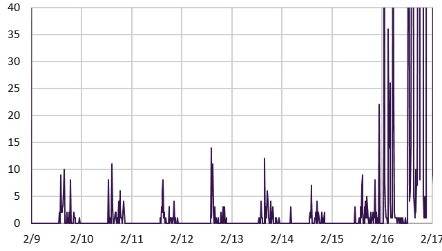
Another thing to watch out for setting your ISR to respond to HIGH/LOW levels rather than RISING/FALLING edges: Level based interrupts will keep triggering as long as that line is HIGH/LOW. This could cause a sketch to run extremely slowly until the interrupt handler is disabled in your program. Even old analog reed-switched based sensors can suffer from this type of issue, as its not uncommon for something like a wind sensor to stop spinning right where the magnet is holding the reed-switch closed.  The thing that makes this choice somewhat tricky is that the most common type of sensor failure I see is one where the alarm stays on permanently.  If you set your interrupt to respond to LOW,  and the sensors starts self-triggering your event counters get pushed up to ridiculously large numbers – so it’s very easy to spot that failure in the data, and by the fact that the logger is usually kept awake till the batteries run dry.  If your ISR responds to FALLING, your counts go to almost zero in the same situation, and depending on the phenomenon you are recording it could be very easy to miss that a sensor problem has developed.  

For more information, there’s an excellent guide to interrupt handling over at the Gammon Forum. Probably the most important thing to keep in mind about using interrupts is that by default all interrupts are disabled once you are inside an interrupt subroutine so that the ISR can’t interrupt itself and create an infinite-recursion situation that over-runs the memory.  But the I2C bus relies on interrupts to function, along with timers and other important things.  So don’t try to change a sensor register while inside the ISR,  just set a volatile flag variable and deal with resetting registers later in the main loop.  The general rule of thumb is: “get in & get out ” as fast as possible, and I rarely have a sensor triggered ISR longer than this:

void  INT1pinD3_triggered()  {   INT1_Flag = true;   }

though sometimes I’ll also detachInterrupt(interrupt#) inside the ISR, to make sure it only fires once for things like button de-bouncing. 

Status registers are usually latched, and have to be reset by the I²C master after they are triggered. DRDY registers are cleared by reading information from the data registers they are associated with.  Most other status registers are cleared by reading the register’s memory location, which also turns off the hardware alarm signals that were mapped from them.  This is different from control registers which always have to be explicitly over-written to with new information to change them. If you are waking up a sleeping data logger based on something like a high temperature alert, you usually read the status registers to clear those alarms before enabling interrupts and putting your logger into a power-down state. Threshold based alarms allow interesting things like burst logging.

In Summary:

A good register map, and the four generic functions I’ve described here

  1. i2c_readRegisterByte
  2. i2c_writeRegisterByte
  3. i2c_setRegisterBit
  4. i2c_getRegisterBit

Should be enough to get a typical I²C sensor running, and you can easily tweak those functions to make custom versions for reading 16-bit registers and/or to mask the cruft out of data pulled from mixed registers.

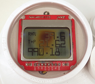
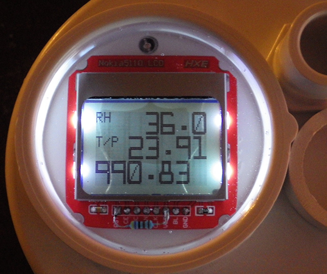
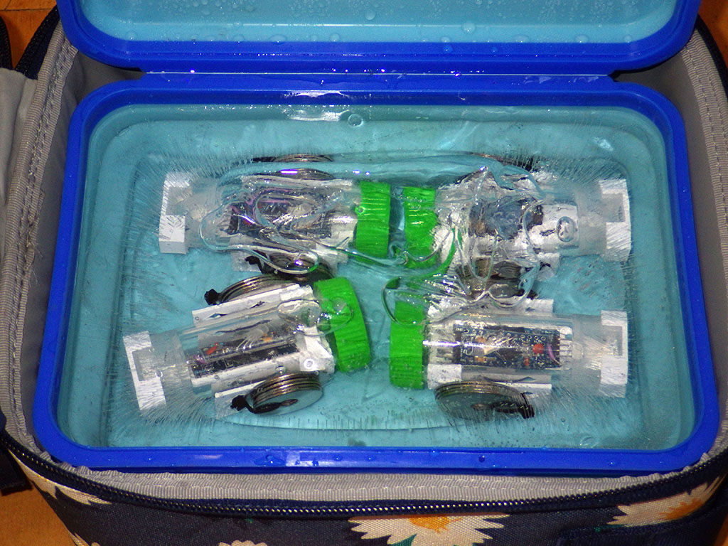
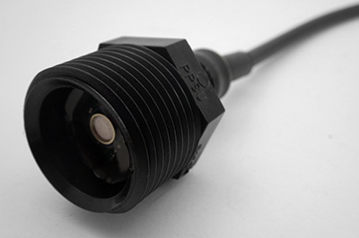
After testing an I2C sensor combination, I pot them in epoxy. Detailed instructions here.

Initializing an I²C sensor is a multi-step process and the correct order of operations is often poorly explained in the data sheet because they are usually written “in reverse”.  Instead of a straightforward list saying “To get a reading from this sensor, do (1),(2),(3),(4), etc.” you find descriptions of the control register bits saying “before you set bit x in this register you must set bit y in this other control register”. When you look up that other control register you find that it too contains a sentence at the end saying “before you set bit y in this control register you must set bit z in this other control register”. So you have to work your way through the document, tracing all those links back until you find the things you were supposed to do first.  Finding the “prime control bit” can be such a time consuming process that it’s not unusual for people who figure out the sequence to wrap it all up into a sensor library so they never have to look at that damn datasheet ever again.

But if you use those libraries, keep in mind that they are probably going to configure your sensor to run at the highest possible bit-depth & data rate, unnecessarily burning away power in applications like data logging which might only need one reading every fifteen minutes.  So the majority of off-the-shelf sensor libraries should be seen as partial solutions, and you don’t really know what else your sensor is capable of until you read through the datasheet yourself.  As an example there are IMU’s out there that will do Euler angle calculations if you simply turn on those functions with the right control register. But libraries for those chips sometimes enable the bare minimum data output functionality, and then do computational handstands to accomplish those gnarly (long) calculations on the Arduino’s modest µC.

In addition there can be useful sensor functions hidden in plain sight, because the datasheet tells you how to turn them on & off, but gives you no clue when to do so. An example here would be humidity sensors like the HTU21D which has an on-chip heating element to help the sensor recover from long periods of condensation, but no status alert that would let you do this automatically. You could just run the heater once a day, but there is also no indication how long the sensor would last if you did that – just some vague references to “functionality diagnosis”. But then some manufacturers (Freescale and Sensirion come to mind…) commit more than just sins-of-omission, breaking away with non-standard I²C bus implementations to lock in customers. The logic there is that if you have to buy the one great sensor that only they make, it’s easier to buy the other four sensors for your device from them as well, rather than juggling low-level protocol conflicts. 

Another challenge when you are working with a new sensor is that Arduino’s C++ environment is not the same as vanilla C in some important ways. So many of the tutorials you find will describe methods that won’t work on an Arduino. Even when the code does compile, there are a number of different “styles” that are functionally identical when they pop out the other side of the compiler, so I’m still trying to wrap my head around the syntax that turns arrays into pointers when they get passed into functionsThat’s why I didn’t mention I2C eeproms in a post about memory registers: almost every multi-byte read/write example out there for EEprom’s uses array/pointer/reference thingies. If you absolutely have to read a series of sensor output registers into an array with a loop, my advice is to just make it a global until you really know what you are doing. And don’t try to store numbers in a char array, because the “temporary promotion” of int8_t’s to 16-bit during some operations can bung up the calculations.

But now it’s time to bring this thing to a close. While I’m still thinking about stuff I wish I’d known earlier, it occurs that a good follow-on to this post would be one about techniques for post-processing sensor data.  There are plenty of useful methods like Paul Badger’s digital smooth, and other code tricks like wrapping those functions in #ifdef #endif statements so those routines only get compiled when a sensor that actually needs them is connected to your logger.

That will have to wait for another day so for now I’ll just sign off with some links. Except for that last ranty bit, I’ve tried to stay out of the I²C handshaking weeds, because when you are up to your neck in bit banging, it’s easy to forget you were trying to measure the water level in a swamp.  But if that’s your thing, there’s some more advanced I²C code examples over at the Gammon Forum, an in depth reference to the Wire library at the Arduino playground , and some troubleshooting tips over at Hackaday.  Its also worth noting that I’ve used bit-shifting to extract bits, and concatenate 16-bit values from 8-bit registers. But you sometimes run into examples where people have uses structs & unions to do those tasks in a much more elegant way.

Addendum 2017-11-04

I wonder how many other sensors I could use this with? And if my pin-toggled oversampling method works on the ATtiny, this might provide better resolution than some commercial sensors; though I guess that would depend on how much I could squeeze into only 512 bytes of SRAM…

Somehow I always seem to run into a bunch of related material the day after I post something to this blog: There’s a cool little project over at Quad Me Up using ATtiny85 to turn an analog light sensor into an I2C slave device.  AN4418 from Maxim explains how to use I/O extenders to connect a compact-flash (CF) cards to the I2C interface, which is something I never thought I’d see. And then theres AN10658 from NXP with a method for sending I²C-bus signals over 100m. My own tests with the I²C sensors just hanging off the Arduino only reached about 20m. Technoblogy has used this ATtiny approach to build an I2C SD card interface and an I2C GPS interface.

Addendum 2017-11-05

Koepel over at the Arduino forum pointed out that the IDE supports some handy macros like bitSet(), bitClear(), and bitRead() that could replace the bit math & masking functions I described above:

byte resisterData = Wire.read();    // byte from register
bitSet(resisterData, 6);                   // change bit 6 to a 1

These handy macros are particularly helpful when setting the internal behavior of the processor on the Arduino board because all the bits in those registers have names that the IDE can translate into actual numbers: 

bitSet (DIDR0, ADC2D);     // disable input buffer on A2 by setting ADC2D bit in register DIDR0

Another highly useful trick is to to use bit_is_set or bit_is_clear macros to poll the value of one of your processors flag registers inside a while loop to create short-duration conditional delays while some process occurs:

while (bit_is_set(ADCSRA,ADSC));   // waits here for ADC conversion to complete

There’s also word(h , l) to combine two bytes, or highByte() and lowByte() to divide 16-bit variables into 8-bit two pieces. These macros may not travel well outside the Arduino IDE, so most programmers avoid using them, preferring to write out the explicit code.

So bitSet replaces x |= (1 << n);  and bitClear can be used to replace x &= ~(1 << n); in in the standard I2C functions I described in the post. Many programmers do not like the code underlying these kinds of compiler substituted macros, so the bit math expressions are far more commonly used because they are generally faster to execute. The AVR can only shift bit positions by one bit per clock cycle (so <<n, takes n clock cycles) but that’s still faster.

There is one other bit-math expression I use frequently, when I want to toggle the state of I/O pins, for example:  PORTD ^= B00001000;  (toggles the state of only bits with a “1” on the right hand side of the expression)  That is a special use case for rapid port switching on the Arduino, rather than for sensor register bits.

Addendum 2017-11-06

I’ve also just found out that there are a small number of sensors there that require a ‘false’ modifier to be used at the end of an I²C transaction:  Wire.endTransmission(false);   This is called a repeated start, and the I2C master does not release the bus between writing the register-address and reading data with Wire.requestFrom();   The sensor responds to the I²C address with an acknowledge at the begin of the I²C transaction, and to each databyte that is written to the sensor, so the error code returned by endTransmission can still be used because it is a test if the I²C address was acknowledged by the sensor.

And there was another I²C quirk mentioned at the Gammon Forum:

“You can’t rely on the slave necessarily sending the number of bytes you requested. If you request 10 bytes, Wire.requestFrom() will return 10, even if only 5 have been sent. For the slave to terminate the communication early (ie. after sending less than the requested number of bytes) it would have to be able to raise a “stop condition”. Only the master can do that, as the master controls the I2C clock. Thus, if the slave stops sending before the requested number of bytes have been sent, the pull-up resistors pull SDA high, and the master simply receives one or more 0xFF bytes as the response…It does not help to use Wire.available() because that too will return the number of bytes requested.”

Another little gem about the I2C interface on the Atmel chips:

“The Twin Wire Interface is virtually identical to the I2C bus. This is actually the bus that the Arduino uses, TWI was developed when the I2C bus was not open source and Atmel did not want to risk a trade name violation. The only major difference between TWI and I2C is that TWI does not support an advanced technique called clock stretching.”

Addendum 2017-11-08

On my page about the DS3231 rtc I describe how to power that I²C chip from a digital pin during bus communication. That trick only works because the chip was designed to gracefully fail over to a backup coin-cell power supply. With other I²C sensors a leakage current might flow into the sensor through the pullup resistors, so you would have to power the bus pullups with the same digital pin to avoid this. And since the internal pullup resistors are enabled by default in the Wire library, you have to disable I²C before you could pin power that I²C device.  Also don’t try to de-power a whole module with decoupling capacitors through a digital output pin as that creates big current spikes and really needs proper switching with a PNP transistor of p-channel FET.  99.99% of the time its better to simply find a sensor with a really low sleep current sleep state that you can enter by setting a control register. The best sensors are ones that automatically go into these low current standby-states whenever they detect no traffic on the I2C bus: then you don’t have to do anything.

Another thing I discovered while working with that RTC was that it had a Wire.begin() call hidden in the library, but I was already starting the I²C bus normally during setup. So without knowing it the I²C hardware was being initialized a second time. As the I²C peripheral registers are set to the same value as in the first Wire.begin() call nothing bad happened. However I can see where it might get’s problematic if you call Wire.begin() accidentally because it was buried inside some sensor library while you were running a data transfer,  and the hardware is re-set to an idle state. 

Addendum 2017-11-09

Most of us are familiar with trying out different libraries to drive a sensor, but I’d be remiss if I didn’t mention that there are also some alternatives to Wire library for I²C. The one that gets the best reviews is the I2C Master Library developed by Wayne Truchsess at DSSCircuits. This lib has a faster throughput and a significantly smaller code size: the original Wire library adds about 796 bytes to your sketch when included whereas Wayne’s I²C library only adds 140 bytes. And it has built-in commands that replicate all of the functions I described in this post. For 16 bit registers Wayne points out:

“Technically when sending bytes to a slave device there is no difference between data and an address. In other words let’s say you have a three byte address and three bytes of data. You could use the write(address, regaddress, *data) by making the first byte of your multibyte address equal to regaddress and then combine the rest of the address and data together into *data.”

and that’s equally true with the wire library. The memory savings alone would be worth exploring, but perhaps I²C Master library’s most compelling feature is a ‘TimeOut’ parameter for all bus coms, which could keep your logger from getting stuck in a while-loop if one of your sensors goes AWOL, though I wonder if it still has the 0xFF problem mentioned above, if the sensor sends less than you requested?  And there are lots of other I2C libraries to explore, and even some updated versions of the lib from DSS.

Addendum 2017-11-10

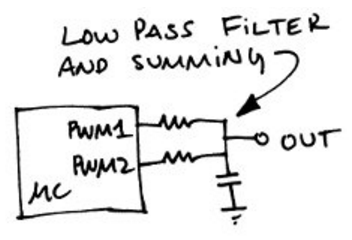
I thought using an ATtiny to convert an analog sensor into an I²C device was a neat trick. But it seems that Andreas Spiess has taken the idea to a new level with three HC-SR04’saccessible through on a single AT.  His youTube video #42 with three Ultrasonic Sensors for Arduino walks through the process, with a vocal track that leaves you thinking Werner Herzog has started doing maker videos. I am impressed with what people achieve using those little processors.  The basic idea of reading an analog signal and turning it into PWM output is common to both amplifiers and sensor applications like light->frequency converters.

Addendum 2017-11-13

The IDE compiler has an annoying quirk when it runs into Wire.requestFrom in those I2C register routines because the compiler throws up warning messages whenever it feels it has to resolve an ‘ambiguous’ call:  (click to enlarge)

 Turns out that requestFrom has two different implementations, one that can take int arguments, and one that takes uint8_t arguments. If you put in something which has no type like a number (or something you declared with a #define) the compiler has to decide which implementation to use. In the case shown above it chose to use the (int,int) flavor even though device address was specified as uint_8 at the start of the function. 

Anyway, to make those warnings disappear, simply cast the two parameters in Wire.requestFrom to either (uint_8) or (int):

And all those compiler warnings will disappear.

Addendum 2017-12-14

Single I2C/SMBus Address Translator for those times when you have an unavoidable sensor bus address conflict. Or you can use an I²C multiplexer like the TCA9548A over at Adafruit which will let you use one I²C address to talk to the multiplexer and tell it which lane you want to enable.

Addendum 2019-06-11:  How fast is the I2C bus?

There’s different ways to think about this question, and most sources quote low-level numbers that make it hard to see the forest for the trees. From the perspective of driving an I2C sensor what you usually want to know is how many times can I capture readings before I have a situation where the bus can’t keep up? (in those cases you usually switch to SPI sensors) 

Nick Gammons I2C page has logic analyzer shots showing the timing for an address byte and single data byte transaction taking ~0.2 milliseconds. A little further down the page he shows another transaction sending the address & two bytes to an 24LC256 eeprom which took about 0.3 ms at the 100 Khz default. And at Saleae.com I found perhaps the ‘most typical’ type of sensor transaction:

You capture a reading from the TMP102 temp sensor shown above with the standard I2C sequence:
1) set the devices memory pointer address to the output register
2) read two bytes of data from the sensor
The sequence takes just under 0.5 ms, so you could achieve ~2000 of these transactions per second.  Add another handshake to ‘trigger each conversion’ and you cut throughput to around 1000 ‘complete sensor transactions’ per second. The TMP102 needs about 25ms to actually take each reading, so the bus is 25x faster at the 100Khz default speed.  However there are plenty of other sensors with output data rates that can approach, or exceed, that 1000 samples per second, and if you are juggling a few of those for a balancing robot or a drone you can create a bottleneck  – and remember the wire library is also preventing your processor from doing anything else for that time.  Fortunately it’s easy to make the bus 4x  faster with the TWBR command. And on 16Mhz Arduinos, I can usually push that to 800 Khz for faster sensors if my wires are short enough.

The DS3231 RTC module we use on our loggers has 4k7 ohm pull-up resistors on the SDA & SCL lines & the Pro Mini adds internal 50k pull ups when the wire library is enabled. I2C sensor modules usually add another 10k each, so our ‘net pullup resistance’ on the I2C bus wires is usually: 50k // 4k7 // 10k = ~3k. With a 3.3v rail that means the devices draw 3.3v / 3k = 1 mA during communication which is fairly normal ( 3mA is max current allowed by the spec) for total wire lengths below 1m. Longer wires and multiple sensors/devices add capacitance to the bus and may require a lower frequency for stable communications. You can change the speed of the I2C bus from its 100kHz default with the TBWR= #; command and the resulting frequency can be derived from this formula:

TWBR = ((mainCPUclockSpeed / BusFrequency) – 16) / 2;       (assumes default prescalar of 1)

You can set any frequency where that formula generating an integer between 0 and 255 however a given CPU frequency cannot generate all possible bus speeds. And the I2C device(s) will set restrictions on the maximum allowed -> the device with the lowest frequency sets your safe upper limit.

The I2C bus speeds you typically see listed for sensors are 100KHz & 400KHz. The RTC module we use in the Cave Pearl loggers has a 100kHz eeprom on board but the DS3231 chip is good to 400 kHz, so on builds where I’m not using the eeprom I will bump the clock up to 400 as most sensors also support the faster speed.  Doing so is a risk because there’s no guarantee that the 100kHz device will not misbehave when exposed to 400kHz traffic – anything from NACKs to bus hangs are possible. It’s also worth noting that on 8Mhz ProMini style Arduinos, pushing the bus clock up to 400kHz (with TWBR=2;) shortens t_low to 1μs, which is below the 1.3 microsecond minimum twi spec. So again you have to test your system thoroughly, and if devices fall of the bus at 400 you can step back to 200kHz. (TWBR = 12;)

So far we’ve gotten away with the faster bus however MOST of the time I actually use TWBR settings to slow down the bus to 50 kHz or even 25 kHz (TWBR = 152; @8MHz) when my wires get longer than 1m, or when multiple sensors have started to cause communication errors. There is no minimum clock frequency in the I2C spec, but regardless of the clock speed the rise time for signals on long cables can’t exceed 1000ns (and the fall time can’t be longer than 300ns – but that’s rarely an issue). Changing to more aggressive 2k2 pullup resistors also helps when you need to hang an I2C sensor off of long wires. We’ve successfully pushed that out to 20m on some of our builds.

Addendum 2020-05-21: Using I2C sensor alarms to interrupt processor sleeping

I just put together a post on the ADS1115 module, which, while it’s not a sensor per se, still provides a good example of how I use ‘DATA ready’ alarms to let me wake & sleep the processor to save power in logging applications.  Many slow I2C sensors have similar ALRT/RDY output pins, so the do{ } while (condition); loops shown in that post are transferable to other sensor modules.

Addendum 2021-01-07:      Resolving I2C address conflict

Another interesting solution to running multiple I2C sensors with the same address:

“Our solution was to use I/O lines on the microcontroller to force the SDA lines high on the devices that we don’t want to address, while the I/O line for the device we’re targeting is set as input (high impedance). This means that only the targeted device matches it’s I2C address and the others ignore any subsequent data.”

Measuring EC ( electrical conductivity ) with Arduino

This post is a summary of my background research into electrical conductivity to serve as a backdrop for my own humble attempts at this interesting measurement challenge. I’m sure there are many other approaches that I’ve yet to discover, and if you know of one please leave a comment so that we can pass that knowledge on to others – Ed.

Obligatory blog-post monkey shot.

Pete & Trish doing profiles with a YSI EXO. As you might imagine, these puppies are pretty expensive. Now that we have A Flexible Arduino-Based Logging Platform to build on,  adding conductivity is our #1 priority. Creating a good drop-profile is an incredibly slow process because you have to wait for the probes to thermally equilibrate and you don’t want to disturb the delicate halo-clines as you pass through them. The last 35m profile I did with a Hydrolab took 2 hours to reach bottom.

The conduction of current through a water solution is primarily dependent on the concentration of dissolved ionic substances such as salt. Since most fresh water derives from relatively clean rainfall, variations in EC provide a way to track the chemical  and hydrological processes the water has been subjected to over time. High amounts of dissolved substances (usually referred to as salinity) can prevent the use of waters for irrigation and drinking, so conductivity ranks as one of the most important inorganic water quality parameters.

A huge number of resources are dedicated to measuring EC and rather than re-hashing all that material, I thought I’d start with links to a few good background reads:

Conductivity, Salinity & Total Dissolved Solids
-discusses the older TDS measurements in parts per million ( ppm ) which makes assumptions about the charge carriers that don’t reflect real world environments.  The conversion factor from EC (which is the thing you actually measure) to TDS changes for different dissolved solids, so instruments from different manufacturers often give you different TDS readings for the same solution, because the companies made different assumptions about what’s in your water.  Because of this confusion, straight EC measurements in siemens have been adopted as the standard by the international scientific community. One siemens is equal to the reciprocal of one ohm (S = 1/Ω)  and is also sometimes also referred to as the mho (℧) in older literature.

Conductivity Theory & Practice
-a white paper that covers basic probe designs, and mentions some non intuitive things like geometry/field effect errors.

Conductivity Sensing at PublicLab.org
-many groups at PublicLab.com have been working on different types of conductivity sensors and their overview page is another excellent introduction to DIY approaches. In fact it’s so good that I will be referring to several of those projects in this post.

Aqueous conductivity is commonly expressed in millisiemens/cm (mS/cm) and natural waters range from 0.05-1.5 mS/cm for freshwater lakes & streams up to about 55mS/cm for sea water. Water up to 3 mS/cm can be consumed, though most drinking/tap water is below 0.8 mS/cm.  Many of the Cave Pearl Project’s installations are in coastal areas where tidally driven haloclines require our instruments to cover that entire “natural waters” range.  Groundwater can vary even more, with measurements being complicated by organic acids and/or significant amounts of dissolved limestone.  Salt water is chemically aggressive and water hydrolyzes above 0.4v, so the probes for high-conductivity environments are usually made of resistant materials such as platinum, titanium, gold-plated nickel or graphite, making them somewhat expensive.

Ways to Measure Conductivity:

There are so many different approaches to measuring EC that it’s taken me a while to digest it all into some working categories.  I expect to build at least one prototype for each of these methods just to see if I can make it work.

Density Based Methods

Refractometers and density based hydrometers are used by aquarium hobbyists. Better quality acoustic doppler flow sensors can also calculate density based on the speed of sound through the water and infer salinity from that. Given then number of acoustic anemometer projects out there, I’m surprised someone has not already adapted the method for underwater applications, though this may be due to the timing limits of the affordable transducers.

Resistance Based methods:

a) Use submerged probes as part of a resistor divider / bridge :
This common approach measures the resistance between two probes using some type of voltage divider. Resistance =1/conductance, which allows you to derive conductivity with your cell K constant since conductivity=(conductance * length)/(area).  AC oscillators are tacked on to reduce electrode polarization, and this forces you to add even more electronics on the output side to convert the signal back to DC for reading. The resistance between the probes changes by several orders of magnitude in environmental waters so different probe surface areas & divider resistors are usually required to cover a significant conductivity range. Above 50% sea water, the resistance between the probes doesn’t change very much, so this method tends to get used more frequently for fresh water environments.

b) Change the pulse frequency of a 555 timer circuit:
You can use resistance between the electrodes as part of an RC relaxation oscillator and then measure the 555’s square wave output frequency to determine the resistance.

This circuit from Thomas Allen’s site provides galvanic isolation, uses AC measurement, and the output frequency varies from about 42 Hz with the probes in air to > 8000 Hz depending on conductivity. You can buy this circuit on pre-made a module for $24  from the EME site.

Circuits and instructions can also be found at at PublicLab.org and there are many good tutorial videos describing 555 based EC sensors on YouTube.  At this point I’ve run into so many projects using this chip that I’d  be willing to bet every environmental sensor I’ve ever heard of could be cobbled together from a few op-amps and a low voltage 555 timer . There are several frequency counting libraries available to help you get started, and if you are ready to sink your teeth into some code, Nick Gammon has produced the some elegant solutions for pulse/frequency timing. Note there are some duty cycle issues  (also see: Schroeder Thesis)

c) Time the discharge of a capacitor through the solution:
Jim Conner’s describes this method in his youTube video at
EC Probes – How they work, and how to build one


A circuit like this might be easy to implement on an Arduino if you can put the internal 1.1v reference onto the comparator that’s also built-in to the 328.  Microcontrollers count time with far better resolution than you get from their ADC’s, but that doesn’t mean there aren’t other issues to deal with. Given that you can try this method with practically no extra circuitry, I will definitely be prototyping a few of these.  Like the 555 based circuits, it will be interesting to see if the method bumps into timing & interrupt handling limits (100 kHz?) when you use it with seawater.

Capacitance based approaches:

You often see capacitance used for liquid level sensors and soil moisture probes, and some of these could be adapted for EC.  To me, the raindrop detection pcb’s you see on eBay have always looked like prime candidates for re-purposing as capacitive sensors.

The circuit described for the Chirp Moisture Sensor uses a fixed resistor and a probe made from PCB traces to create a low pass filter whose cutoff frequency changes with capacitance,  which is affected by the material around the probe surface. This filters an 1-8MHz square wave and the output voltage is accumulated other side of simple diode peak detector circuit for reading. Cheaper versions of this sensor use a 370kHz square wave at the input end which is about the fastest pulse you can get from a cheap 555. Unfortunately that’s not quite fast enough for most salinity work which usually works with MHz.

You can also vary 555 timer output frequency by changing the capacitor in the tank circuit, or create more complicated oscillator circuits. No matter which cap-based method you use, the supporting electronics have to be located near the sensor – because just about any length of wire will add enough stray capacitance to throw off measurements. Because you need large resistances to compensate for the small (50 – 500 pF ? ) capacitance of the probe, you are essentially creating an antenna. Unfortunately pF levels are too small for the traditional charge/discharge timing methods which work so well in the nF to uF range.

The resulting RC filter time constants make these methods much more suitable for the air/water application which changes the probe capacitance by almost an order of magnitude (50-400pF) , with more dissolved ions acting like wetter soil.  Once the probe is submerged the output delta for fresh vs salt water with the RC filter approach is MUCH smaller. (say 400pF to 450pF …ish?) Using the probes capacitance as part of an LC oscillator would give you better discrimination of small changes,  as MCU’s can count frequency reasonably well.

Another thing to keep in mind with the RC filter method is that common ceramic capacitors have some of the worst thermal coefficients and aging effects imaginable so your pulse source is likely to drift as well. Plastic film capacitors using Polyphenylene Sulfide (PPS ±1.5%) or Polypropylene (CBB or PP ±2.5%) have much better tempcos, and having a digital capacitance meter on hand is probably a good idea, though most won’t even measure down to the 1pF range you’d need with small probes.

Potentiometric (4 electrode) Methods

Four-electrode cells uses two “driver” pins to place an electric field across two other “reading” pins that lie between them: 

This paper describes a DIY 4-probe sensor that was used for soil moisture sensing, and you will find quite a few articles using potentiometric methods over at IEEE and Sensors ALSO see Design of sound speed profiler -Water Parameter Sensor (2017 Master thesis) by Shaban, A, University of Oslo –  which describes building a four electrode sensor with Arduino

Nokia/Apple audio jacks came to mind as soon as I saw this diagram, and they might be available with gold plating.  4-electrode methods often measure the voltage between the read pins, which is divided by the exciter pin current to determine the solution’s impedance = 1/conductance.  To obtain the conductivity, the conductance is multiplied by the cell constant of the inner poles. Tracking the pin current lets you compensate for fouling on the plates, and the method can cover a wide range of conductivity. Like inductive methods, this approach tends to work better as the concentration increases. 

Inductive Methods

The conductivity measurement is made by passing an AC current through a toroidal drive coil, which induces a current in the solution. This induced solution current, in turn, induces a current in a second coil, called the pick-up toroid. The amount of current induced in the pick-up toroid is proportional to the solution conductivity. You get industrial grade performance out of this non-contact method in many different types of solutions, but you also need industrial amounts of power the drive the sender coil so it’s hard to implement on the kind of power constraints you see on stand-alone data loggers.  Inductive sensors require a 3 inch radius from any other surface (bio-fouling?) and you see this pretty clearly in the ‘donut on a stick’ sensor heads. It occurs to me that you see very similar components in a wireless charging system, but there’s a lot of devils hiding in those details – like shielding, etc.  It might be possible to press one of the production line proximity sensor chips into service for a low power solution, or simply try measuring changes in inductance due to the presence of salt water.

Off-the-shelf Solutions for Arduino:   (using 2-Electrode Resistance Methods)

TransparentSinglePixl
Atlas Scientific Conductivity Kit
A complete solution including calibration solutions, a range of probes and code libraries. All parts also sold separately: interface boards are ~$35 & EC probes come in around $120 each but they are durable enough for continuous long term submersion.  I2C data transfer is supported, so resolution is not limited to the Arduino’s ADC.  Whitebox labs Tentacle Shields ($35-$110) provide up to four galvanically isolated channels for full hydroponic rigs. Stand alone BNC carriers for $10. The notable Open CDT project makes use of these sensors. See Jonas Auråen’s Thesis for a comparison of Atlas sensors to a commercial CTD.
$200
CN0349 Conductivity Measurement System
The EVAL-CN0349-PMDZ has total error less than 1% FSR after calibration. The digital output is fully isolated eliminating ground loop interference. Even if you are using a different circuit at the sensor, its work looking at how they did that.  Thanks for the tip about this one from Joshua Girgis: “Its designed to work as a benchtop sensor but one can easily wire it up to the i2c lines on an Arduino. The code is a little cumbersome but I have it working for taking temperature and conductivity measurements for sea water.”  Update 201907 :  Joshua has released an Arduino library for this board on his GITHUB.
$45
Gravity: EC Sensor Kit for Arduino (K=1)
Another complete K=1 kit solution, but the probes are not robust enough for long term submersion so several people replace the stock probe with the 208DH which is available on eBay for $35. Arduino ADC reads voltage.  The KnowFlow project uses the full set of DFrobot boards. DFR also has an inexpensive TDS kit, which cfastie has been testing over at publiclab.org
$70
Vernier CON-BTA EC probe
This 5v K=1 probe covers 0-20,000 μS/cm  in the high range, and the analog voltage output is read by the Arduino ADC. You need an inexpensive adapter board for the BTC connector, and they provide a basic library. One key feature is built in hardware temperature compensation with a 10k thermistor in the probe head. My tests show this reduces the usual 2% / °C reading variation down to about 0.5%/° C, so you still need to do your own calibration to get higher accuracy. Like Atlas Scientific, Vernier has many other interesting sensors that are Arduino compatible. (Much cheaper on Ebay for older stock)
$115
EC/pH Transmitters
This company offers a range of physically bulky turn-key solutions, with the $70 entry level unit claiming 0-5000 μS/cm (fresh waters) and continuous monitoring. Arduino ADC reads voltage. ~$200 units support PH with isolation.
$70-250
Sparky’s widgets MiniEC
An indie who makes several other useful sensor breakout boards, including PH. You have to build or locate your own probes, though they use a standard BNC connector like most EC probes.  Arduino ADC reads voltage output. Works with many of the inexpensive probes you find on Alibaba – some of which look remarkably like the probes used by Atlas?
$24
EC-Salinity Probe Interface by Ufire
Designed around an ATtiny configured as an I2C slave, probably using the cap-discharge method.
$14.50
Hanna HI 73311 (K=1) Replacement probes
In the past we’ve used used these epoxy&graphite probes from Hanna DIST5 (HI 98311) and DIST6 (HI 98312) testers, which connect to a standard male audio jack.  You can also re-purpose one of the Vernier ABS/graphite probes if you get a used one cheap on eBay, and the Vernier probes have a 10k NTC thermistor built in, which you can read with a divider. The best completely DIY probes I’ve ever seen are the concentric electrodes built by Camilo Rada with epoxy & graphite rods.
$55
Comercial Standard Solutions
For fieldwork, it’s often easier to transport the dry packets, and mix them on location.  Atlas sells calibration sets, but at the twice the cost of standards when you buy them in larger volumes.  You can find recipes for homemade calibration solutions at Reefnet Central and PublicLab. For a classroom situation, it’s much cheaper to mix secondary “lab standards” in larger quantities, and then test the resulting solutions with a commercial probe that’s been calibrated against commercial solutions. 5.566g of dry NaCl in 1 litre of distilled water will create an ~10,000 μS/cm solution, which you can dilute down for lower concentration standards.
$14/500ml

This photo from Bitnitting gives you a sense of the physical space needed for the Atlas breakouts and a ‘mini’ form factor Arduino.

Hydroponics hobbyists have putting these kits to good use over the years with notable examples like the long running forum thread on Billies Hydroponic Controller, and the well documented adventures over at the Bitnitting Blog.  The people at OpenCTD and other academic projects have put the Atlas boards into real world deployments.

But to me these commercial solutions still leave you stuck with those expensive electrodes which sometimes cost more money than you would pay for a used 4-pole device. More annoying is the fact that those cell constants do not line up with my goal of measuring the entire “fresh” to “marine” range with one sensor, thought if I could extend it a bit the K=10 probe comes close.  This is illustrated by the following graph from Andy Connelly’s Blog which is worth digging through as he has posted lots of other interesting material on calibration, reproducibility, signal detection, etc. 


Of course the cell constant changes as your probes get older and dirtier, so you have to re-calibrate them with standard solutions just about every time you want to take a new reading. I’m pretty sure I will end up making my own probes, probably out of Nichrome 80 wire as the vaping fad has made it common on eBay. Some have had good EC results with gold plated PCB traces. Feedback on the Arduino.cc forum suggests that Platinum-Rhodium Thermocouple Wire is another good option.  I’ve also been wondering about Ag/AgCl which is highly resistant to seawater and is commonly used for non-polarizing electrodes in medical/bio applications. (EKG electrodes?) It might also be a good idea to cobble together a DIY magnetic stirrer, based a PC fan and an old hard drive magnet

DIY 2-Probe EC Circuits

The easiest circuits to build yourself are the 555 timer oscillators, but there are plenty of quad-opamp solutions out there for people comfortable with a breadboard. The oldest example I’ve seen is this one by M. Ahmon from the Sept 1977 issue of Electronics magazine which uses the resistance of the solution to modify opamp output:

This circuit uses the first stage of the quad opamp in a Wien-bridge oscillator, reducing errors caused by electrolysis with a 1-kHz signal that gets attenuated by the solution’s resistance before it reaches the driving amplifier A2.  Pot P1 controls oscillator amplitude, and P2 adjusts gain of A2.  A3-A4 form a precision rectifier giving output voltage equal to absolute value of input voltage. This one chip solution seems to have been the basis for many of the current EC projects on the web, including these two exceptionally well documented examples:

Octavia’s EC/TDS/PPM Meter On Limited Budget

Daniel Kramnik’s Digital Salinometer Project

Similar circuits can be found on the breakout modules from Sparky’s Widgets and DFrobot . Using the solution’s resistance in the feedback divider controlling an op-amp is a neat idea, but having only one opamp there imposes hard limits the range you can measure with a given K value probe. There is a more advanced multi-opamp approach over at pulsar.be that can step over several decades.

On more recent EC projects I’m seeing single supply RRIO opamps for the oscillator & gain stages, which are easier to integrate with battery operated Arduino’s. (though any dual supply opamp can be used as a single supply in a pinch; since voltage is relative the opamp doesn’t know whether V- is a negative voltage or ground) To keep using an AC signal, this requires a virtual GND at 1/2 VCC, but the integration also gives you the option of getting rid of the oscillator entirely, since you can use PWM output as your source.

This is beautifully illustrated by the circuit from bhickman’s Conductivity & Temperature Meter over at PublicLab:

Ranging is accomplished with the (red) bank of R1 resistors, and (yellow)R2’s 5/6 can be substituted in for the probe (R8) with those known resistances can be used to track drift. The AC–DC converter stage is built with precision peak detectors. I think this is the best voltage divider approach I’ve seen to date.  To simplify things a bit, you might replace that output stage with an RMS-DC converter; though I’ve not seen any breakouts for those, and I hate working with raw SMD parts.

Sources of Error: 

Even with a clever circuit like the one above you still need to address things like temperature compensation before you get an accurate, repeatable, and stable device. Electrical conductivity measurements are typically referenced to 25 °C using standard temperature compensation factors (α). The conductivity of natural waters exhibit strongly nonlinear temperature behavior, though in practice linear correction factors are most frequently used.  NaCl-based solutions typically have a temperature coefficient (α) of 0.02-0.0214 (~ 2% change/degree C). So to convert your “ambient” conductivity measurement into 25°C “specific” conductivity, the simple linear conversion is:

EC25=ECambient /[ 1 + α (tambient – 25) ], α= 0.02

Field effect errors are significant, causing read errors if bare 2-pole electrode get within 2-5 cm of the solution container: which will completely mess up your calibration and cell constant determination. This is one reason that virtually every EC probe is encased inside a plastic shroud of some sort. That causes field effect errors too, but at least its the same error every the time, rather than one that varies depending on how far you are from the edge of the beaker. Four probe methods also require a fixed volume of solution between the driver electrodes, so the shroud provides that.

Grazing through the hydroponics forums shows plenty of people struggling with cross-sensor interference.  Most notably when conductivity probes affects the accuracy of a PH probe in the same tank.  Any time two devices are immersed in the same environment differences between them can generate ground loop voltages and induce currents which degrade the readings and exacerbate corrosion.  Sometimes you can address these issues with optical or I2C isolators. One helpful contributor at Arduino.cc suggests:

pH electrodes are very high impedance devices and the cabling and connectors are all important – even flexing a decent cable will distort the readings…. Ground loops are the enemy of pH and any other specific ion electrode. I used them a lot in difficult situations and the most trouble-free solution is always to put a buffer op amp (FET type) as close to the electrode as possible – some commercial electrodes come already equipped. Find a decent op amp like the old MAX406, high impedance techniques like PTFE insulators or simply keep the input pin off the board. Modern FET’s take single-sided supplies and run at better than 2-microamps – a 3.6-V lithium cell will give you in excess of 5-year’s trouble and ground loop -free operation. Once you have buffered the signal, you can use any cable you like. As a bonus, you can convert a pH electrode into an ammonia electrode by separating the water from the electrode with PTFE tape as used by plumbers.”

Well, I think that covers most of the stuff I had in my notes, and hopefully gathering it all here saves someone else from burning away that time. I have been experimenting with conductivity quite a bit lately, and I think I might have  come up with an analog approach that will allow people to play with conductivity on shoestring budgets. I just have a little more calibration testing to do before I let that one out of the bag  🙂

Addendum 2018-12-06

Folks working on EC might want to check out our tutorial video showing how to build underwater connectors  ( part of the 2017 logger build series )   Near the end of that video we mount an Atlas EC probe on a long cable for a student project. 

Addendum 2020-04-30

Recently got a tip from someone over at the Prince William Sound Science Center, who mentioned a paper with a fascinating hack of an Onset light & temp logger which turns it into a stream intermittency sensor:

Robust, low-cost data loggers for stream temperature, flow intermittency, and relative conductivity monitoring     Zeigler (2014), Chapin, T. P., A. S. Todd, and M. P.
Water Resour. Res., 50, 6542–6548, doi:10.1002/2013WR015158.

While somewhat crude, the circuit also provides a rough estimate of relative changes in conductivity. I suspect this would only work in freshwater, but if the underlying circuit was reading a garden variety CdS photo detector then this approach would make a good student project an a DIY logger too.

Tutorial: Calibrating Oversampled Thermistors on an Arduino Pro Mini

Selecting a thermistor (& series resistor) value

Most of the material you find on thermistors makes the assumption that you are trying to maximize sensitivity and interchangeability. But oversampling gives you access to enough resolution that sensitivity is less critical, and interchangeability only makes sense if you are putting them in a product with good voltage regulation. In that case, precision thermistors like the ones from US sensor are a good option, but according to Campbell Scientific, that choice has other knock-on implications:

“The resistors must be either bought or selected to 0.02% tolerance and must also have a low temperature coefficient, i.e. 10 ppm or preferably 5 ppm/°C.”

Like many better quality components, these resistors are often only available in SMD format, with minimum order quantities in the thousands. If you use a typical 1% resistor with a T.C. of 50 ppm or more, you could introduce errors of ±0.1°C over a 50°C range, which defeats the point of buying good thermistors in the first place.

Still, if I was only building a few sensors, I’d spring for the good ones. But now that I have oversampling working on the Arduino, I’d like to add a thermistor to every logger in the field, and the mix of different boards already in service means I’ll have to calibrate each sensor/board combination. That time investment is the same whether I choose a 10¢ thermistor or $10 one.

Power consumption is also important, making 100kΩ sensors attractive although I couldn’t even find a vendor selling interchangeable thermistors above 50k.  A low temperature limit of 0°C (the units are underwater…) and putting 1.1v on aref to boost sensitivity,  requires a 688k series resistor, which is far from the 1-3x nominal usually recommended:

Here I’ve overlaid an image from Jason Sachs excellent thermistor article at Embedded Related, which shows I will only see about ⅓ of the sensitivity I would get if I was using a 100k series resistor. I highly recommend reading Jason’s post, despite the fact that I’m ignoring almost all of his good advice here…  🙂

Using the internal band-gap voltage as aref improves the ADC’s hardware resolution from 3.22mV/bit to 1.07mV/bit.  This trick gives you a extra bit of precision when you use it at the default 10bit resolution, and I figured I could do it again to compensate for the lost sensitivity due to that big series resistor.

In return, I get a combined resistance of at least 700k, which pulls only 4.7μA on a 3.3v system.  Such low current means I could ignore voltage drops inside the processor and power the divider with one of Arduino’s digital pins.  In practical terms, burning less than a milliamp-second per day means adding a thermistor won’t hurt the power budget if I leave it connected to the rails all the time; which you can only do when self-heating isn’t a factor.  This is quite handy for the bunch of old loggers already in service out there, that I want to retrofit with decent temperature sensors. 

Even 100 ohms of internal chip resistance would produce only 0.5mV drop,  so depending on your accuracy spec,  you could use 16-channel muxes to read up to 48 thermistors without worrying about cable length.  There aren’t many of us trying to connect that many temperature sensors to one Arduino, but using a 100k  thermistor also makes me wonder if you could mux a bank of different series resistor values, pegging the divider output at it’s maximum sensitivity over a very large temperature range.

What is a reasonable accuracy target?

Combining 5¢ thermistors & 1¢ metfilms, means my pre-calibration accuracy will be worse than ±1°C.  Cheap thermistor vendors only provide nominal & βeta numbers, instead of resistance tables, or a proper set of Steinhart-Hart coefficients. So I might be limited to ±0.4°C based on that factor alone.  And it took me a while to discover this, but βeta values are only valid for a specific temperature range, which most vendors don’t bother to provide either.  Even with quality thermistors, testing over a different temperature range would give you different βeta values.

In that context, I’d be happy to approach ±0.1°C without using an expensive reference thermometer.  Unfortunately, temperature sensors in the hobby market rarely make it to ±0.25°C.  One notable exception is the Silicon Labs Si7051, which delivers 14-bit resolution of 0.01°C at ±0.1°C.   So I bought five, put them through a series of tests,  and was pleasantly surprised to see the group hold within ±0.05°C of each other: 

Temps in °CCompared to what I usually see when I batch test temperature sensors, this is pretty impressive for an I2C chip that only cost $9 on Tindie.

Ideally you want your reference to be an order of magnitude better than your calibration target, but given the other issues baked into my parts, that’d be bringing a gun to a knife-fight. 

So my calculations, with oversampling, and the internal 1.1v as aref become:

1) MaxADCReading                  (w scaling factor to compensate for the two voltages)

= ( [2^(OverSampledADCbitDepth)] * (rail voltage/internal aref) ) -1

2) Thermistor Resistance        (w series resistor on high side & thermistor to GND)

= Series Resistor Value / [(MaxADCReading / OverSampledADCreading)-1]

3) Temp(°C)                                  (ie: the βeta equation laid out in Excel)

=1/([ln(ThermResistance/Tnominal R)/βeta]+ [1.0 / (NomTemp + 273.15)]) -273.15

Seeing the error in my ways

I knew that the dithering noise would have some effect on the readings, and all the other source ADC of error still apply.  Switching to 1.1v reduces the absolute size of most ADC errors, since they are proportional to the full scale voltage. But the internal reference is spec’d at ±0.1v; changing the initial (rail voltage/aref voltage) scale factor by almost 10%.  Since all I needed was the ratio, rather than the actual voltages, I thought I could address this chip-to-chip variability with the code from Retrolefty & Coding Badly at the Arduino.cc forum.  This lets Arduinos read the internal reference voltage using the rail voltage as aref.

I started testing units in the refrigerator to provide a decent range for the calibration:

Si7051 in blue vs 100K thermistor in red. The sensors were held in physical contact. ADC was read with 1024 oversamples providing approximately 15bit resolution. Temps in °C.

and strange artifacts started appearing in the log.  The voltage readings from both the main battery and the RTC backup battery were rising when the units went into the refrigerator, and this didn’t seem to make sense given the effect of temperature on battery chemistry:

Si7051 temp. in °C on the left, with the RTC backup battery (V) in green on the right axis. The CR2023 is monitored through a 2x10MΩ divider, using the 3.3v rail as aref. The large number of ADC readings needed for oversampling has the side benefit that it lets you read very high impedance dividers, but by the time you reach 10Meg ohms, you pick up 5-10 points of noise in the readings. Which is why that coincell voltage line is so thick.

I think what was actually happening was that the output from the regulator on the main board, which provided the  ADC’s reference voltage for the battery readings, was falling  with the temperature.

When I dug into what caused that problem, I discovered that temperature affects bandgap voltages in the opposite direction by as much as 2 mV/°C.  So heating from 0°C to 40°C (and some loggers will see more than that…) reduces the 328P’s internal reference voltage by as much as a tenth of a volt. In fact, bandgap changes like this can be used to measure temperature without other hardware.  This leaves me with a problem so fundamental that even if I calculate S&H constants from a properly constructed resistance table, I’d still be left with substantial accuracy errors over my expected range.  Argh!

Becoming Well Adjusted:  (Beta ain’t better…)

These wandering voltages meant I was going to have to use the internal voltmeter trick every time I wanted to read the thermistor.  It was mildly annoying to think about the extra power that would burn, and majorly annoying to realize that I’d be putting ugly 10bit stair-steps all over my nice smooth 15bit data. This made me look at that final temperature calculation again:

Temp(°C) =
1/([ln(ThermResistance/Tnominal R)/βeta]+ [1.0 / (NomTemp + 273.15)]) -273.15

which I interpret as:

 =fixed math(  [(ADC outputs / Therm. nominialR ) / Therm. βeta]  + (a #) ) – (a #)

Perhaps tweaking the thermistor’s nominal value (which I only know to ±5% anyway) and changing the (fictional) βeta values would compensate for a multitude of sins; including those voltage reference errors?  Then I could just pretend that (rail/aref) scaling factor had a fixed value, and be done with it:         (click image to expand)

So in my early tests, all I had to do was adjust those two constants until the thermistor readings fell right on top of the reference line.  Easy-peasy!

Well …almost. Repeat runs at 15bit (1024 samples) and 14bit (256 samples) didn’t quite yield the same numbers.  Applying the best fit Nominal and βeta values obtained from a 15bit run to 14bit data moved the thermistor line down by 0.05°C across the entire range (and vice versa). So the pin toggling method I used to generate the dither noise introduces a consistent offset in the raw ADC readings.  While that doesn’t completely knock me out of my target accuracy, I should generate new calibration for each oversampled bit depth I intend to use. It’s still good to know that the dithering offset error is consistent.

Throwing a Big Hairy Fit

I was pleased with myself for the simplicity of the Nominal/βeta approach for about two days; then I pushed the calibration range over 40° with a hot water bath:

Blue=Si7051 , Orange = 100k NTC thermistor.  1024 oversamples = ~15bit. Temps in °C.

This gave me targets at around 40, 20 and 5°C.  But no combination of Nominal & βeta would bring all three into my accuracy range at the same time.  Fitting to the 20 & 40 degree data pushed the error at 5°C beyond 0.2° :             (click image to enlarge)

…and fitting to 20 & 5, pushed the 40C readings out of whack.  After more tests I concluded that tweaking βeta equation factors won’t get you much more than 20° of tightly calibrated range. 

My beautiful plan was going pear-shaped, and as I started grasping for straws I remembered a comment at the end of that Embedded Related article

“… in most cases the relationship between voltage divider ratio and temperature is not that nonlinear. Depending on the temperature range you care about, you may be able to get away with a 3rd-order polynomial or even a quadratic..”

Perhaps it was time to throw βeta under the bus, and just black-box the whole system?   

To find out, I needed to prune away the negative temperature regions where the voltage divider had flat-lined, and remove the rapid transitions since the thermistor responds to changes more quickly than the si7051:                 (click image to inflate)

Then it was time for the dreaded Excel trend line:

Ok, ok. I can hear people inhaling through their teeth from here. But with 15 sigfigs, Excel seems like the height of luxury compared to the constraints in μC land.  I wonder what an advanced modeler like Eureqa would have produced with that dataset? 

The trick for getting workable constants is to right-click the default equation that Excel gives you, re-format it to display scientific notation, and then increase the number of displayed digits to at least six.  

Some people use the LINEST function to derive these polynomial constants but I’d advise against it because seeing the raw plot gives you a chance to spot problems before you fit the curve. When I generated the first Temp vs ADC graph, the horizontal spread of the data points showed me where the thermistor and the reference thermometer were out of sync, so I removed that data.  If I had generated the constants with =LINEST(Known Y values, X values^{1,2,3,4})  I could have missed that important step.

For the following graphs, I adjusted the trend line to display to nine insignificant digits:     

Blue =Si7051 reference, Orange is that 20&40 best fit from tweaking Nominal & Beta values, and the yellow line is the 4th order polynomial from Excel.   Temps in °C. (Click to embiggen)

It took a 4th order polynomial to bring the whole set within ±0.1° of the reference line and 5th order did not improve that by much.  Now I really have no idea where the bodies are buried!  And unlike the βeta equation, which just squeaks in under the calculation limits of an Arduino, it’s beyond my programming ability to implement these poly calcs on a 328 with high bit depth numbers. I certainly won’t be writing those lunkers on the bottom of each logger with a sharpie, like I could with a pair of nominal/βeta constants.

This empirical fit approach would to work for any type of sensor I read with ADC oversampling, and it’s so easy to do that I’ll use it as a fall back method whenever I’m calibrating new prototypes. In this case though, a little voice in my head keeps warning me that wrapping polynomial duct tape around my problems, instead of simply using the rail voltage for both aref & the divider, crosses some kind of line in the sand. Tipping points can only be predicted when your math is based on fundamental principles, and black-boxes like this tend to fail dramatically when they hit one.  But darn it, I wanted those extra 1.1v aref bits! Perhaps for something as simple as a thermistor, I’ll be able to convince the scientist in the family to look the other way.

Making the Steinheart-Heart equation work

Seeing that trend-line produce such a good fit to the temperature data, made me think some more about how I was trying to stuff those system-side errors into the βeta equation, which doesn’t have enough terms to cope.  By comparison, the Steinheart-Heart equation is a polonomial already, so perhaps if I could derive some synthetic S&H constants (since my cheap thermistors didn’t come with any…), it would peg that ADC output to the reference line just as well as Excel did?

I rolled the voltage offsets into the thermistor resistance calculation by setting the (rail voltage/internal aref) scale factor to a fixed value of 3, when in reality it varies from slightly below to slightly above that depending on the board I’m using:

1) MaxADCReading                  (w scaling factor to compensate for the two voltages)

=(2^(OverSampledADCbitDepth) * (3)) –1

2) Thermistor Resistance        (w series resistor on high side & thermistor to GND)

= Series Resistor Value / ((MaxADCReading / OverSampledADCreading)-1)

and I went back to that trimmed 40-20-5 calibration data to re-calculate the resistance values. Then to derive the constants, I put three Si7051 temp. & thermistor resistance pairs into the online calculator at SRS:

Note: There are premade spreadsheets that you can download which will generate S&H constants, or you can build your own in Excel  [see pg6 of this whitepaper]  There’s also coefficient calculators out there in C, Java, etc. if that’s your thing.

With those Steinhart-Hart model coefficients in hand, the final calculation becomes:

3) Temp °C =1/( A + (B * LN(ThermR)) + (C * (LN(ThermR))^3)) – 273.15

and when I graphed the S&H (in purple) output against the si7051 (blue) and the 4th order poly (yellow), I was looking at these beauties:

and that fits better than the generic poly;  nearly falling within the noise on those reference readings. With the constants being created from so little data, it’s worth trying a few temp/resistance combinations for the best fit. And this calibration is only valid for that one specific board/sensor/oversampling combination;  but since I’ll be soldering the thermistors permanently into place, that’s ok.  I’m sure if I hunt around, I’ll find a code example that manages to do the S&H calculations safely with long integers on the Arduino. 

So even with cheap parts, oversampling offsets & bandgap reference silliness, I still made it below ±0.2°C over the anticipated temperature range.  Now, where did I put that marker…

Addendum 2017-04-27

Just a quick note to mention that you need to tape the thermistor to the si7051 sensor so they are held in physical contact with one another. The thermistors are tiny & react to temperature changes much faster than the si7051’s which have a much larger thermal mass because of the breakout board they are mounted on. So the temp/resistance pairs don’t match up as well as they could if the sensors are in physical contact with one another.

Addendum 2017-06-05

With 1.1v aref in the mix,  my 15bit oversampled resolution on those 100k thermistors varies between 0.002 and 0.004°  from 20-40°C. But I was throwing the bandgap aref in just to see if I could still make it work. From a calibration point of view, it’s better to better to use the rail voltage on aref, and remove that 3x ratio from the MaxADCReading calculation.  This will lower the resolution to somewhere between 0.006 to 0.012C with a 688k series resistor unless you bump up the oversampling to compensate. In addition to tripling my noise/toggle-pin current, how much extra power do I have to pay to get that resolution back if I’m using the 3.3v rail as aref?

In my oversampling experiments, I found that the Arduino ADC works well at 250 kHz, delivering just under 19230 ADC readings /second. For the purpose of estimation, assume the Pro-mini style boards I’m using draw about 5mA during the sampling time, and I take a reading every 15 minutes (= 96 readings per day) :

15bit= 1024 reads/19230 r/sec =0.053s*5mA =0.26 mAs*96/day=~ 25 mAs/day
16bit= 4096 reads/19230 r/sec = 0.213s*5mA =1.00 mAs*96/day= ~102 mAs/day
17bit= 16384 reads/19230 r/sec = 0.852s*5mA =4.26 mAs*96/day= ~408 mAs/day

so it would cost me another 385 mAs/day to reach a resolution slightly better than I was achieving with the 1.1v bandgap on aref. Given that a typical AA battery runs about 2000 mAh = 2000 mAh*3600 sec/hour =~7,000,000 mAs, it would be quite a while before that breaks the power budget.  Removing the ratio dependency also means that your S&H constants are for the resistor/thermistor pair only, making that calibration independent of what system you connect them to.

Using an Rnominial=100k series resistor would give about the same effective resolution boost as going to 17 bit, but that option costs you more power if you are leaving the thermistor powered all the time:

3.3v / 780k combined resistance  = 4.23μA x 86400 sec/day  = 366 mAs/day
3.3v / 200k combined resistance  = 16.5μA x 86400 sec/day  =  1425 mAs/day

You can power the thermistor from a digital pin, but since I’m already using digital-pin toggling to generate noise for the oversampling, I still need to test if I can combine pin power for the sensor with my oversampling technique. It’s possible that the thermistor bridge needs to be powered by the more stable rails, while I’m shaking aref inside the processor, because if the voltage on the divider started moving in sync with the ADC noise, the dithering noise will effectively disappear, and my oversampling would stop working.

Even before doing this test, I have a sneaking suspicion that 100k series vs. oversampling vs. other techniques  will end up converging on the same effective resolution in the end. And I’ll even hazard a guess that the point of diminishing returns is somewhere around 0.001°C, since that’s what you see offered by quite a few high-end temperature loggers.

Addendum 2017-09-24

Just posting an update about pin-powering the thermsitor dividers while using the 3.3v rail as aref: everything works, but as I suspected you need to stabilize the thermistor with a small 0.1uF capacitor or the dither noise vanishes.  This also requires you to take the RC time constant into account, waiting at least 5x T  for that parallel cap to charge before you start reading the divider. You can sleep the processor during this time, since I/O pin states are preserved.

Degree Celsius vs. Time with lines offset for easier visual comparison:  The blue line is over-sampled output from a pro-mini clone reading a 100k Thermistor /100k series voltage divider. Aref was set to the 3.3v rail, with a 100nF capacitor in parallel with the thermistor on the low side.  This RC combination has a time constant of ~10 milliseconds.  A 0.12 mA pin-current provided sufficient noise for dithering 1024 readings: to deliver an effective resolution of ~0.0028° at 24°C.  For comparison, the red line is the output from an I2C si7051 sensor on the same logger, with a resolution of 0.01°C.

So using a 100k series resistor with 3.3v aref really does deliver the same effective resolution as the 680k series/1.1v aref combination, and it does not suffer the problem of bumping into the aref voltage at a certain temp.  I’m using 100k termistors so the pin resistance (~40 ohms) will introduce less than 0.05% error over the range; though this pin-drop error would be higher for therms with lower Rnominal values.

Since I’m using cheap eBay 100k’s and a host of other no-name components, I have to calibrate each logger/thermistor/O.S. bit-depth combination.  This isn’t much of a burden for the overall workflow, since I always give new loggers a shake-down run, in fact, I usually do a fast sampling burn for at least a week before considering a unit ready for deployment:

That Degree vs Time image above was an excerpt from a calibration run like this. I’ve found that Freezer (morning)->Fridge (afternoon)->Room (overnight) is easier to manage than the reverse order, and gives enough time at each temperature to deal with thermal lag differences between the thermistors and the reference sensors.

As before, when I do the thermistor resistance calculation I make the assumption that everything in the system is behaving perfectly (which is obviously not true). So errors from things like pin drops, temp. coefficients, ADC gain, etc., are getting rolled into the S&H constants.  Essentially, I’m eliminating a host of different corrections in exchange for the interchangeability between sensors that I might have if I took all those factors into account individually. This makes it easier to standardize the code , and is a reasonable trade-off for loggers that I won’t be seeing again for several years, but if I have to swap some components at that time, I’ll need to do  another calibration.

The other factor is that every time you introduce one of the many possible corrections, you necessarily limit your final output to the stability, resolution, or number of significant digits in that correction.  In one case the limits of my rail voltage reading method produced random spikes in the record whenever that factor in the calculations had a brief toggle:

Note: spike errors are also diagnostic of calculation errors due to over-running your variables. The difference is that variable overflow problems are not random like the one shown above. They repeat regularly whenever the data passes some threshold in the calculation.


In more extreme cases this noise shows up as a overall thickening of the output from correction factors that toggle their relatively low-rez bits more frequently.  As an example I did some runs where I took a Vcc reading with the internal bandgap trick, and rolled that into the thermistor calculation to improve the accuracy. the net result was that the 4-digit Vcc reading placed a limit on the final output so that there was no “effective difference” in the thermal resolution between oversampling at 15bit & 16 bit because that VCC correction had been included.  (Note: You’ll run into this problem more often if you change aref voltages and forget leaving enough time for the aref capacitor to stabilize…)

The Arduino’s reference (and ADC) do not have a zero tempco.  However, if you make the “perfect” regulator/band-gap/ADC assumption the only limits placed on your resolution are the significant figures in your S & H constants.  Even so, there are so many other factors at play here, that I suspect that you can’t use my pin-toggle oversampling technique to push the Arduino’s ADC much past 16 “effective” bits before some other limitation occurs. Then there’s the issue of long term drift of the various components and the fact that it takes over 200ms each 16-bit reading; adding about 20 seconds of CPU run time to my logger’s daily duty cycle.  Remember that my goal here was a dirt cheap temp sensor that I could add to every logger with a modest accuracy in the 0.1-0.2C range.  If you need both resolution and accuracy, then you should switch to ratiometric measurements, with an instrumentation amp like the INA826, and a 24bit ADC.

Addendum 2017-11-05

Looks like Sensirion’s new STS35 has ± 0.1°C accuracy like the si7051 I’m currently using as a calibration reference. Since the Steinhart-Hart” equation has a built-in error of ~0.1°C and the si7051 ref is ~0.1°C, that might get me into the ball park of ±0.25°C accuracy.  Hopefully that shows up on Tindie soon.  Of course, it’s important to remember that we’re miles away from a real ITS-90 level calibration with a triple point cell.

Addendum 2018-03-14

I recently found out about a method using temperature-sensitive liquid crystals as thermal calibration references at 55, 75, and 90 deg°C. These were custom-made by Hallcrest UK (www.lcrhallcrest.com) and apparently the transitions were sharp enough to resolve 10 mK..?  That’s still a bit rich for my blood, but I also thinking about experimenting with virgin coconut oils (on amazon) which melt at ~24 °C  – the actual value is imprecise, but hopefully will remain constant for a given batch of oil.  So could provide a nice melting point plateau…we will have to see…

Addendum 2018-06-10

Still hunting for a good method to provide nice thermal plateaus for the calibration runs covering >30°C of range. The refrigerator gives a nice 5°C point, and of course room temp is easy, but getting that third calibration point up at ~35°C is a bit trickier because I want that peak to be long and slow.  In the winter that’s available on the house radiators, but during the summer I don’t have a ‘slow’ dry heat source in the right range.  I’ve been following some threads suggesting that you can convert a regular water bath into a “dry-bath” with copper coated BB shot, or aluminum pellets. Both would be a heck of a lot cheaper than lab grade dry bath beads, though for an application where i am simply looking for a slow temperature ramp (so hot & cold spots don’t matter) sand or rice might suffice to provide the thermal mass I need. And I could use an old bath from eBay for the job – these sometimes sell for as little as $25 if they have surface rust on them.  Or perhaps I could hack the temp sensor on a charity shop crock-pot to keep the temp really low….

Addendum 2019-03-25:

I’ve been developing a new method for reading thermistors with the Input Capture Unit on pin D8. Micro-controllers count time much more precisely than ADC’s measure voltage, so this new approach delivers more resolution than 16-bit oversampling in about 1/10th the time & power. The ICU also lets you use a single diode as a temperature sensor.

Give your Arduino a high resolution ADC by Oversampling with noise (from a toggled pin)

Thermistors are really twitchy, so you need to put them inside a big lump of thermal inertia before you start.

The slightest breeze makes glass bead thermistors jitterbug like crazy, so put them inside something with a decent amount of thermal inertia before you do any oversampling experiments. Otherwise thermal noise could make it look like your dithering is sufficient for oversampling, when it’s not.

While I was figuring out how to read thermistors with our Arduino based data loggers, I came across claims that you can improve the resolution of any Analog-to-Digital converter with a technique called oversampling & decimation. I had already doubled the number of ADC bits covering my target temperature range by powering a thermistor divider from the rails and using the internal 1.1v as the analog reference.  And my gut feeling was that aref-based ADC bits were somehow better than any I could synthesize, but I was still curious to see if I could add over-sampled bits to the ones obtained with the bandgap trick.

At first bounce, the method appeared to be incredibly simple, to get n extra bits of resolution, you need to read the ADC four to the power of n times.  Generally you have to add three extra bits (43= 128 samples) to see approximately an order of magnitude improvement in your real world resolution. With thermistor dividers, you typically get about 0.1°C from the default ADC readings, and 128 samples bumps that to 0.012°C.  Taking (46= 4096) samples would bump that up to ~0.0015°C which, as the saying goes, is good enough for government work… 

I usually over-sample one power more than needed for my target resolution, so I’d use for four extra bits to be sure of that order of magnitude improvement, which requires the sum of 44= 256 readings:

uint32_t extraBits=0;    // use an unsigned integer or the bit shifting goes wonky
for (int k = 0; k< 255; k++) {
extraBits = extraBits +analogRead(AnalogInputPin);
}

which is then decimated by bit shifting right by n positions:

Oversampled ADC reading = (extraBits >> 4);

This combination lets you infer the sub-LSB information provided there is enough random noise in the signal for the lowest ADC bits to toggle up and down while you gather those readings. But without the noise, all of the original ADC readings are the same, and the oversampling technique does not work.  To show you what that kind of failure looks like, here is oversampling & decimation being done over 4096 readings with no noise or dither signal applied to a 10k NTC thermistor divider read with 1.1v aref:

This is an example of oversampling with no dither signal being applied. So this is the nul result

These are readings from a 10k NTC thermistor divider, and I’ve offset these records from each other by 0.1° for easier comparison. The one-shot ADC readings of the thermistor bridge in purple are converted to °C, as are 4096 sample readings at the default 125kHz(ps64) in grey,  250kHz(ps32) in orange and 500kHz (ps16) in green. With such a large number of samples, the averaging produces some smoothing whenever the raw ADC readings near a transition point, but if you see “rounded stair steps” like this then oversampling is not working properly  the curves shown above are all FAILURES.

Some microprocessors have enough jitter in their readings to use oversampling technique with the natural toggling of the least significant bit.  A few brave souls have even tried to improve the AVR’s crude internal temperature sensor with the technique.  But most of the time, there is not enough naturally occurring noise, and you need to add a synthetic dithering signal to force those LSB’s to toggle.  This is mentioned from time to time in the forums, with a number of references to AVR121: Enhancing ADC resolution by oversampling, but I found frustratingly few implementations using an Arduino that were described in enough detail for me to replicate them.  Most of the technical docs were focused on audio applications, and I was quickly buried under thick mathematical treatments warning me not to interpret the Effective Number of Bits (ENOB) as Effective Resolution (what?), and describing a host of other quid pro quos like signal synchrony.

This is qwerty's original dither circuit from the freetronics forum post at: http://forum.freetronics.com/viewtopic.php?t=5589#p11126

This is Qwerty’s original dither circuit from the freetronics forum. If you are using an UNO, this works well. Of course the ratio between the 5v rails, and the internal bandgap reference,  means you also have extra ADC resolution available without oversampling if you use the 1.1v aref trick, but oversampling gives you more bits for your effort.

About the only useful thing I got out of most of those refs was the apparent consensus that any synthetic dithering signal needs to be at least 2x the voltage per bit on your ADC (although you can use a larger dither signal without causing problems) and triangular dither signals work better than natural noise.  But few of those references said anything about extending ADC resolution, as they were primarily focused on improving the ADC’s signal to noise ratio.

And then there was the fact that several of the older hands seem to dismiss the whole idea as not worth the bother because you had to add so much additional circuitry that using an external ADC was a simpler, cheaper approach.  In fact the subject triggered the closest thing to a flame war I’ve ever seen at the usually staid Arduino playground.  So I was about ready to give up on the idea when I came across a post by user QWERTY at the Freetronics forum explaining how he used a simple RC filter to turn an Arduino’s 480 Hz PWM output into a 9mv p-p triangular dither, which he patched directly into the center of a thermistor bridge.

Yes it is possible to add a jumper on the Aref line of a pro mini.

You can patch into the aref line on a Promini by soldering a jumper to the end of the little stabilizing capacitor.

Holy cow! A solution that only needed a few cheap parts and couple of pins. What the heck were those other guys gassing on about?   My first thought was to try to take the output from Qwerty’s RC filter, and put it onto the Aref as they did in AVR 121.  A compelling idea since putting the dither directly on aref means you don’t have to interfere with the sensor(s), and the same dither circuit would work for all of the analog inputs.  In addition, I was using large resistance voltage dividers to monitor Vbat without wasting power and the high impedance forced me to add a capacitor to feed the ADC’s sample and hold input.  I knew that low esr cap would kill any dither signal that was applied directly to the main battery divider.

fig35avr121

This L-P filter from AVR121 ap-note that everyone mentions works great, but modifying the circuit to give you other aref base voltages is a bit of a pain.

I tried many different combinations, but I never saw the voltage on aref that I expected.  It took ages to discover that ~32k of internal resistance gets connected when you place an external voltage on the aref line, and that forms a ‘hidden’ voltage divider with your circuit. Grrr…

I did eventually get a few of those circuits working, but that internal resistor  seemed  to be slightly different on each board I tried, and I didn’t know if it was going to be stable with temperature, time, etc.  Another important issue was that I was switching from the internal 1.1v aref to read the thermistor, back to using the default 3.3v for other readings during the logger operation. So to put the dither directly into aref meant I would also need some way to modify the baseline aref voltage on the fly.  

Tune the resistor ratio, and roll PWM2 duty cycle and I'm pretty sure this circuit form Open Labs would give you variable Aref voltages.

Tweak the resistors & this circuit could give you variable arefs AND dithering.

I suppose that a truly elegant solution would do that with a PWM/RC filter circuit generating a variable DC voltage, and using a second PWM input to add the much smaller dither signal.  You could tune the dithers pk-pk amplitude to match the adjusted LSB, by the way you varied PWM2’s duty cycle (or by using the tone function)  during the readings.  But working that out would probably give me a host of other problems to resolve (esp. with timing) and I was after a simple solution, with the smallest number of parts.  So I eventually abandoned the “dither on aref” approach.

This brought me back to Qwerty’s method of putting the triangular dither signal on the center of the thermistor bridge. My first task was to change that RC filter: lowering the 9mv swing on his 5v circuit to match the much lower 1.1mv/LSB you get when using the internal bandgap as aref.

The power supply ripple calculator at OKAWA Electric was a perfect tool for this job:

oklowpassfilter

3.6mV was just an arbitrary 'close enough' point for me to start at as I had those components in the parts bit already.  But if you see random flat spots in your oversampled readings at the default ADC speed, then try increasing the ΔV pk-pk of your dither signal a little bit.

3.6mV was just an arbitrary ‘close enough’ point for me to start at as I had those components in the parts bin already.  But if you see random flat spots in your oversampled readings at the default ADC speed, then try increasing the ΔV pk-pk of your dither signal a little bit.

…which revealed that a 4.7MΩ/0.1uF RC combination would take the 3.3v 480Hz PWM on D6 and bring it down to  ~3.6mv peak to peak.  I immediately  hopped over to the Falstad circuit simulator to see the see how this worked.  To simulate an Arduino’s positive PWM, I used a 3.3v square wave source with an offset of 3.3v.  The little 10nf coupling cap prevents the pins DC voltage from affecting the thermistor reading, and the 2k2 bridge resistor prevents the dither signal from being grounded out when the 10K NTC thermistor resistance gets very low.  One of the coolest features of this simulator is that if you build a circuit with it, you can export a web link (like the ones above) that rebuilds the circuit instantly, so you can compare different versions simply by keeping those links in your log.

rcrisetime_png

The RC settling time is shown on the Okawa calculator’s step response graph, or you can watch the voltage rise on the scopes in Falstad by restarting the simulation with the buttons on upper right.

I love using Falstad for “What happens if I do this?” experiments. Of course these usually fail, but in doing so they show me that there are things about a circuit that I still don’t understand.  One thing that gave me a lot of grief when I started working with these  dithering circuits was that I did not appreciate how much time they need to stabilize.  This gets worse if you start disconnecting the thermistor  divider to save power between readings.  

So although I was getting smoother curves, and resolution that looked about 10x better than my raw ADC readings:

excerpt from 1024 oversampled temp record on Arduino ADC with triangular dither , 100kthermistor

Here I’ve converted these 1024 sample curves to °C , and artificially offset each curve by 0.05° from the next to it for easier visual comparison. The one-shot 10bit ADC reading at the default 125kHz (ps 64) is in purple, with other ADC speeds:  250 kHz (ps32) in orange,   500 kHz (ps16) in green, and 1 MHz (ps8) in blue.

At the height of my coupling capacitor lunacy I produced this beast, thinking I could simultaneously read a reference bridge, and correct away any offsets.

At the height of my coupling capacitor infatuation I produced this beast, thinking that if I could simultaneously add dither to a reference bridge I would be able to correct away ADC offset & gain errors, along with the offset caused by the dither signal, at the oversampled bit depth. But all those capacitors added artifacts to the readings when I reconnected GND through that mosfet, producing weird spikes in the data if I took readings less than two minutes apart (?)

…in any set of successive readings, the offset between the oversampled readings and the one shot ADC reading was changing depending on how long the PWM had been running.  No problem I thought, I’ll just throw in another coupling cap to block that slowly rising DC voltage, and connect the ADC input on the thermistor side. Unfortunately replacing the 2k2 bridging resistor with a coupling capacitor forms a high pass filter with the thermistor itself, forcing you to increase the size of the cap to raise the filters cutoff frequency above your 480Hz PWM. But that increases your RC time constant so then the filter starts to act like a differentiator: distorting your nice triangular dither signal (see pg12 of this pdf), and in some cases even reverting it back to the original square wave you started with… Argh!

So the result of all that trial & error is the basic PWM->triangular dither method works well, but you have to wait for the RC filter’s output to stabilize or it messes with your accuracy. And you still end up with a small offset in the ADC readings of 1/2 your dither signals peak to peak, because the original PWM square wave can only be positive.

Crank it up

But no one wants to see a data logger burning away precious milliamp-seconds just twiddling its PWMs!  With guidance from Nick Gammon’s fantastic ADC page, I had already been messing around with pre-scalars to increase the temporal resolution of my UNO DAQ.  I was further encouraged by this line from AVR120    “For optimum performance, the ADC clock should not exceed 200 kHz. However, frequencies up to 1 MHz do not reduce the ADC resolution significantly.  …and there were some tantalizing hints that cranking up the speed might also increase the internal noise enough to make oversampling work better. 

To figure out how fast your ADC is running:

System clock / prescalar = ADC clock,  ADC clock /13 = # of ADC reads/second

The core clock speed on 3.3v promini style boards is 8 MHz, providing:

8 MHz / 64 = 125 kHz /13 ticks    = 9600 /sec      (256 reads =27.6ms, 1024 =106ms, 4096 =426ms)  (default) 
8 MHz / 32 = 250 kHz /13             = 19230 /sec     (256 reads = 13ms,  1024=53ms, 4096=200ms)
8 MHz / 16 = 500 kHz /13             = 38000 /sec     (256 reads = 6.7ms, 1024=27ms, 4096=108ms)
8 MHz /   8 = 1 MHz /13                 = 76900 /sec     (256 reads = 3.3ms, 1024=13ms, 4096=53ms)

Your sensors output must be stable while you gather these samples and this limits what kind of phenomenon you can measure. At the default ADC clock speed, trying to add six extra bits of resolution (46 = 4096 readings) means you can only capture about 2 samples per second. That’s pretty darned slow for data acquisition! In fact, it’s so pokey that some people implement ring-buffer schemes to provide access to an oversampled reading at any time, without having to grab a whole new set of samples. A neat trick if you are continuously monitoring a sensor that changes slowly, and you have enough memory to play with.  Given the powers of 4 relationship between the different bit depths, it’s easy to see how you might hop-scotch through shorter 64 sample readings, and then combine those into a sort of rolling average version of a 256 sample reading if you don’t have quite enough ram for the full ring buffer approach.

enobs

My tests agree with the results posted at Open Labs. You can only push the ADC clock so far before you lose hardware bits, and this defeats the resolution gained from oversampling by making your accuracy worse. You can see this effect in the 1MHz line in the previous 1024 sample graph. Most AVR’s are lucky to get 9 ENOB’s at their default settings.

200 kHz is the ‘official’ ADC speed limit for 10 bit accuracy, but I didn’t see any  significant difference between oversampled readings taken at the default 125kHz clock (ps 64), and those taken at 250kHz (ps 32).  At 500kHz (ps 16) the readings were good most of the time, but during rapid temperature transitions the readings started to ‘wiggle’ as though the dither signal was occasionally dropping out.   At 1MHz (ps 8) the curves wander around quite a bit, and I was seeing errors of ±0.05°C or more with some prolonged flat spots starting to appear. What’s interesting about this is that the triangular dither RC filter puts a capacitor across the thermistor, which should reduce the input impedance seen by the ADC and allow for faster readings.  But this did not reduce the 500kHz wiggle / 1MHz wandering in any of my test runs.  The ATmega328P datasheet quotes 2 LSB’s (typical) of absolute accuracy with an ADC clock at 200 kHz, but 4.5 LSB’s (typical) at an ADC clock of 1 MHz. There is no point in pushing clock speeds if the accuracy gets worse by that much in the process.

So you can always double the ADC clock speed for oversampling, but going up to 500kHz depends on whether you can live with the accuracy errors that prescalar creates.  Those 500kHz wiggles become less evident as you progress from 256, to 1024, to 4096 readings, but that’s probably just an artifact of the smoothing.  The other thing to keep in mind is that one full cycle of the 480Hz PWM takes  ~2 milliseconds, but 256 readings at a 500kHz ADC clock takes only 6.73 milliseconds – so there is a high probability that dither signal synchrony issues creep in at the higher ADC speeds to produce offsets that affect the entire curve. Ideally you’d want the time you spend gathering the over-samples to be an exact multiple of the dither cycle time…

Let’s make some noise!

Hotter prescalars cut the oversampling time down dramatically, but I could not see how to avoid that RC settling time, which seemed to require about 50-60ms of PWM operation before the offsets became tolerable.  So I went back to the proverbial drawing board and asked myself, what if forget about the triangle dither signal, and try oversampling with some sort of random noise?

The first hurdle there was:  How was I going to generate this noise if the processor was already busy taking ADC readings?  The beauty of PWM based dither is that it just chugs away in the background, leaving the processor free.  As usual, Nick Gammon provided an elegant solution to this problem with code on his page about interrupts which showed how to read the ADC asynchronously:  

// Note: Before calling this function, I change to the internal 1.1v aref and set the ADC prescalars
// but you can leave them at the defaults: see: https://www.gammon.com.au/adc for more details
volatile int adcReading;
volatile boolean adcDone;
boolean adcStarted;
unsigned int  adc_read;

unsigned long asyncOversample(int readPin, int extraBits)

    {
int i=0;int j=0;
int var=256;                                  //default is 4bits worth of oversampling
if(extraBits == 5){var=1024;}
if(extraBits == 6){var=4096;} //I’ve only included three options here, but hopefully you see the pattern
unsigned long accumulatedReading = 0;
adc_read=analogRead(readPin);   // a throw away reading to connect the ADC channel
//delete me:  simply as spacer
pinMode(5, OUTPUT); digitalWrite(5, LOW);  // set the pin you are toggling to OUTPUT!
//delete me:  simply a spacer a spacer comment for blog layout
while(i < var){    // asynchronous ADC read from  http://www.gammon.com.au/interrupts
  if (adcDone)
  {adcStarted = false; accumulatedReading += adcReading; adcDone = false;i++;}
  if (!adcStarted)
  {adcStarted = true; ADCSRA |= bit (ADSC) | bit (ADIE);}

  PORTD ^= B00100000;  // XOR toggle D5 w green LED & 30k limit resistor (see  below for details)
}   // end of while (i < var)

pinMode(5, INPUT);digitalWrite(5, LOW);  //turn off the toggle pin
if(extraBits == 4){accumulatedReading=(accumulatedReading >> 4);}  // Decimation step for 4 extra bits
if(extraBits == 5){accumulatedReading=(accumulatedReading >> 5);}  // 5 bits
if(extraBits == 6){accumulatedReading=(accumulatedReading >> 6);}  // 6 bits
return accumulatedReading;
}   //end of asyncOversample function

ISR (ADC_vect)     // ADC complete ISR needed for asyncOversample function  
  {  adcReading = ADCL | (ADCH << 8);adcDone = true; }

(NOTE: copy/pasting code from WordPress blogs is almost guaranteed to give you stray/302 errors because of hidden shift-space characters that the layout editor inserts. If that happens to you, look at the line your compiler identifies, delete all the spaces and/or retype it slowly using only ASCII characters.)

Next I had to generate the noise itself. People use Zenner diode breakdown to produce random numbers, and connecting an analogue input to the collector of a run-of-the-mill transistor, with the emitter grounded and base open also creates noisier randomSeed(); input. But thought I would see if I could generate noise inside the processor, since there seemed to be no end of people complaining about the Arduino’s ADC in the forums. However when I actually tried to do this by connecting pull-ups,  changing I/O settings, an every other kind of processor toggle I could think of, I got nothing.  That ADC was solid as a rock until I started flipping the pins connected to the external indicator LED.   Even then, the early results were wildly inconsistent, with the same code producing good oversampling on one unit, but not another.

Like the hidden resistor problem, it took me a while to notice that the random bunch of LEDs on my breadboard test units had significantly different forward voltage drops from one LED the next, and from one RGB color channel to the next.  Once I realized how much that was affecting the results,  it didn’t take long to determine that that the noise generating sweet spot (with 1.1v aref…) was somewhere around 0.04mA of pin current:

An example of oversampling with pulsed pin current of 0.038mA to generate ground line noise.

One-shot ADC reading shown in purple, with oversampled readings taken at 125kHz (ps64 default)  in grey, 250kHz (ps32) in orange, 500kHz (ps16) in green. All readings are converted to °C, and I’ve offset these curves for clarity, as they would otherwise be on top of one another. You can clearly see the PS16 wiggle as the temperature falls, and the sharp eyed will notice there are still offsets between the different runs which were all taken in quick succession. These seem to be more apparent in the longer slower oversampling runs than they are in the the shorter faster ones… darn it…

Unlike triangular dither techniques, which will tolerate a fairly large ΔV, this noise based method stopped working (ie: flat spots started appearing) when the toggled pin current went below 0.02mA, and the curves became pretty scratchy above 0.06mA  indicating there was too much noise.  That’s a fairly tight range, and it was sheer luck that the 30k limit resistor I was using on my indicator LED’s brought me close enough to spot the effect.  So my current target is ~0.04mA of pin current for 1.1v dithering. And there was nothing special about the LED being there either, as tests using a simple 82.5KΩ resistor from the  PORTy ^= _BV( PDx/PBx );    toggled pin to ground produced good results.  This is pure conjecture on my part, but if you assume the mosfets on the I/O pins have about 40Ω of internal resistance with 3.3v control, then 0.04mA pin current would produce a voltage drop of ~1.6 mv – which is suspiciously close to the 1.1mv/LSB resolution of the ADC with the internal bandgap set as aref.  That puts this dither noise right in the 1-2x volts/bit recommendation from the literature.

rtcdividerreadings

Here I’m oversampling with 1024 readings from a 2x10MΩ divider which cuts the voltage of the RTC’s backup coin cell in half. 250kHz (psS32) in orange, and 125kHz(ps64) in grey. These are the raw readings with aref set to the default 3.3v and there is no capacitor on the divider. This is far beyond the 10k input impedance the ADC was designed for, but I think the many repeated readings you do with oversampling helps the 14pF sample&hold caps do their job. At this resolution, the CR2032 seems to be acting like another temperature sensor …(?)      UPDATE: So this actually was the battery responding to temperature rather than the dithering method, which does not work with the rail voltage on aref unless you add a cap to the voltage divider.

This pin-toggling noise technique is not exactly a one size fits all solution, and the exact current required to induce ADC bit toggling will vary depending on which board you are using, and especially on which capacitors are being used smooth the output from the voltage regulator.  So you will have to noodle around a bit to find the correct resistor value to use for your particular Arduino.

I’d start with a resistor value that draws enough current to give you a voltage drop on the digital pins mosfet that is close to 2x your ADC’s mV/LSB resolution. With 3.3v as aref (so 3.22mV/bit), I would use a pin resistor of  about 27.5k for a pin current of 0.12mA which should cause a pin vdrop of ~4.8mV.  Given that limit resistor for the pin13 LED is usually around 1K, you might be able to toggle that on-board LED to generate this dithering noise without adding any extra components.

With 5v control logic, the mosfets controlling the digital pins are more fully turned, so the pin resistance is somewhat lower; around 25-30 ohms. With 5v on aref your resolution is about 4.88mv/bit, and the dither resistor would have to pull around 0.39 mA to shake the rail with a vdrop twice that mv/bit, so the dithering resistor would need to be somewhere around 12.8 kΩ.  

On new builds I will measure the forward voltage drop of the indicator LEDs and change the limit resistor to give me the current through those I need to generate dither noise. That way I don’t need to any new digital lines for the oversampling process, though this will entail checking every LED, as there is significant vf variation between batches.  The blue channel on the RGB’s I have lying around have a vf of ~2.473v, so 0.827v will be left for the resistor to cover with a 3.3v rail.  To achieve a target pin current of 0.12mA the limit resistor (for that blue LED) would have to be 0.827v/0.00012mA = 6.89kΩ.

This method is also critically dependent on the tiny capacitor stabilizing the aref voltage. When I tried it on the units I had left over from the ‘dither on aref’ experiments, the pin toggling method did not work if the aref stabilizing capacitor had been removed.  I also suspect that the voltage on the capacitor ‘adjusts’ to the noise pulses over time, which might be causing the 0.02C difference between the 256 & 1024 readings shown above. So there could be another settling time issue if you take a large number of over-sampled readings in rapid succession. Larger caps stabilizing the rail voltage on breakout boards may also affect the method. And then there’s the fact that within a processor it is practically impossible to ensure, ALL timers, interrupts, and other processor activities operate randomly with respect to the timing of the ADC conversions. So you can be sure we are generating ‘noise’ that is not random, so there will be offsets created that you will need correct for.

This technique will work with any resistive sensor being read with a simple voltage divider, provided there are no capacitors nearby to smooth out the noise which is vital for oversampling.  I’m not going to pretend to understand all the math behind it,  but it’s probably safe to say you can add somewhere between 2-5 extra bits of resolution to your ADC before the technique suffers from limiting problems somewhere else.  Although the 256 sample curves are a bit gritty, you can make that many samples with the ADC clock at  250kHz in ~13milliseconds, which doesn’t impact the power budget much. If something interesting starts happening with your sensor, you can enable another bit or two of resolution on the fly to zero in on the phenomenon.

Overall, the results from oversampling with toggled-pin noise are not as smooth as the curves you get with a well tuned triangular dither, but I’m happy to trade that last bit of synthetic resolution for a method that’s instantly available on all of the ADC inputs.  The icing on the cake is that I won’t have to add any extra circuitry to use oversampling on the fleet of loggers already on deployment, because all I have to do is toggle the indicator LEDs they already have on board, since their limit resistors were already in the current range I need…YES!

Addendum 2017-04-26:

I’ve moved on to calibration, and in the process I learned that regulator & bandgap voltages change a fair bit with temperature. So it’s probably not a good idea to use the internal bandgap on aref with this oversampling method if you want thermistors calibrated over a wide temperature range. But I did it anyway.

In those tests I used a 688k series resistor with a 100k thermistor, so I was far from divider’s optimum of Rseries=RTnominal. I was taking 1024 oversamples, adding five oversampled bits to ADC, and I was using the internal bandgap voltage on aref, which added another bit.  Since I was on the tail end of the divider sensitivity curve, the effective resolution changed quite a bit over the range: the output shifted from ~0.0018°C/bit at 20°C, to about 0.0038 °C/bit up at 40°C. This is better resolution than some people achieve reading thermistor bridges with the 16bit ADS1115, though gathering all those readings means I can only capture 18 samples per second – even with the ADC clock at 250kHz.

I have a long way to go before I reach the accuracy levels you see at the geotechnical high end, but I think that’s still good for readings with a humble Arduino ADC!

Addendum 2017-09-24:

Several people have contacted me about their attempts to get this ‘pin-toggling noise’ method working with different Arduinos at higher voltages.  If I had to summarize the kernel of understanding that was missed in the unsuccessful cases it is this:

If you jiggle one part of the system with noise – stabilize the other part.

It does not matter if the noise shows up on aref, or on the sensors output, so long as it is not present in the same form on both.  With the bandgap 1.1v as aref, you can rely on that to be the stable side, so you want the voltage divider with your sensor not to have a capacitor on it, since the sensor side needs to shake by ±2 LSB volts when the pin is toggling. The internal reference is slightly different on each individual chip (from 1V to 1.2V), so you’ll also need to “calibrate” if you go this route. Don’t forget to throw away the first reading after changing the analog channel, and if you have a high resistance voltage divider, add a one ms delay after that first analog read.

If you use the rail voltage as aref (the default) with an un-stabilized voltage divider then your pin toggling current shakes the aref ground in perfect synchrony with the ground line on your sensor, and no matter how many samples you read & decimate you will never get beyond the 10 bit resolution of the ADC. So to use the rail as aref when oversampling you need a small (around 0.1uF) capacitor across the lower half of your thermistor divider so the sensors input to the ADC becomes the stable side. It’s also a good idea to remove the little 0.1uF stabilizing capacitor that’s normally present on the aref line, since it’s whole purpose is to prevent aref from jittering. 

Degree Celsius vs. Time with lines offset from each other for easier visual comparison:  The blue line is over-sampled output from a pro-mini clone reading a 100KΩ  NTC Therm/100KΩ series voltage divider. Aref was set to the 3.3v rail, with a 100nF capacitor parallel to the thermistor on the low side.    A 0.12 mA pin-current provided sufficient noise for dithering 1024 readings, delivering an effective resolution of ~0.0028° at 24C. For comparison, the red line is the output from an I2C si7051 sensor on the same logger, with a resolution of 0.01C.

The question of which side should be treated as stable comes into play when you want to over-sample analog output from more complex sensor circuits. If the circuits on a sensors supporting breakout board are already doing a good job of stabilizing output, say with feedback, caps and some sort of buffer at the end of an amplification cascade, then you have no choice but to set aref to the rail voltage and shake that. I’ve had success with this approach and a complex sensor circuit on a 5v Nano, by pulsing a pin connected to ground through a 12KΩ resistor (~ 0.4 mA of pin current).

No matter which side you shake, everything else in your system is feeling this noise to some extent, and this may cause issues with sensitive sensor IC’s, or with micro-controllers other than the 328p.  Of course, the higher the aref you use, the more of a voltage swing you need to introduce for sufficient dither. The effect of the pin current is also being limited by capacitance distributed throughout the system, which varies from board to board, so this is definitely a “try it an see” method: when it works it really works, producing smooth curves with no hint of the underlying 10-bit ADC peaking through(Most of the time I get acceptable oversampling results toggling the green channel of a three color RGB indicator LED with ~24k limit resistor but that is somewhat dependent on the LED’s forward voltage. When in doubt, use a smaller limit resistor to increase the pin current – and check the actual value with a DMM)

If you see any flat spots or rounded stair steps in your temp. data, especially in areas where the changes are occurring slowly over time, then you know the dithering is not working:  

This is an example of the natural noise problem: oversampled (blue line) thermistor readings achieved high bit depths the refrigerator (left), but developed flat spots in the room (right) where the changes were happening more slowly. This was a test run with the noise circuit disconnected,which I followed with run using the same code +noise applied so I could compare the two. Doing two runs (with & without dithering) is good general approach to use when testing a circuit that uses oversampling.

Any natural signal variation over your sampling interval will make it look like your generated dithering noise is sufficient for oversampling, when it is not.  The photo above shows how that this test is almost impossible to do in the refrigerator, because the natural on/off cycle of the compressor generates enough change/time to make oversampling work without dithering. 

With stabilizing capacitors on the voltage divider you also have the trickier problem of spotting the influence of the RC time constant when you only power the voltage divider during readings.  Oversampling before the cap is fully charged will provide more than enough change in the readings to hide inadequate dithering.  In fact, if you scale the capacitor/series resistor combination, and sample over the 3T-5T interval after applying power, you get reasonably good oversampling results with no other noise in the system.  In some ways, using RC rise time is better than pin toggling when you are using the rail as aref, since it does not have to fight against the other capacitance distributed around the system to produce a delta on the ADC readings.  I’d use this rather than pin toggling with aref=rail  if it weren’t for the fact that capacitors can have the worst variation coefficients of any electronic component you are ever likely to run into.

Garden variety Y5V ceramics vary by up to 82% over their rated temperature range, and even the X7R’s that most engineers use vary by +/-15%. I might be able to calibrate that thermal variation away, but for environmental monitoring the drift over time is a much bigger problemwith caps commonly loosing 10-15% of their rating over the first year (~8900 hours) of operation. There are stable NPO rated ceramic caps out there, but they are only available in relatively small pF sizes, and a good 0.1uF NPO cap will set you back about $7 each even if you buy them in quantity, so that part alone costs more than a decent IC based temperature sensor.

Plastic film capacitors have much better thermal coefficients: Polyphenylene sulfide (PPS ±1.5%) or Polypropylene (CBB or PP ±2.5%)A quick browse around the Bay shows those are often available for less than $1 each, and the aging rate (% change/decade hour) for both of those dielectrics is listed as negligible. The trade off is that they are huge in comparison to ceramics, so you are not going to just sneak one in between the pins on your pro-mini. 

For most rail-as-aref situations, Qwerty’s PWM based dither method (mentioned at the beginning of this post) is a more robust way to dither with cheap ceramic caps, since it can tolerate significant variation in a way that does not affect your accuracy that much – but you still have to keep an eye on the circuit settling time. 

Addendum 2017-10-15:

Just came across AN2668 from STMicroelectronics which sums the input signal and triangular dither signal through an op-amp before sending it to the ADC:

Still seems like a lot of work to me, although that ap-note does have me wondering if the pin-toggle dither noise is actually Gaussian…?

Addendum 2019-03-25:

Pin Toggled Oversampling has been delivering solid results for more than a year now in the field, but I’ve recently been developed a new method for reading thermistors with the Input Capture Unit on pin D8. Micro-controllers count time much more precisely than ADC’s measure voltage, so this timer based approach delivers more resolution than 16-bit oversampling in about 1/10th the time & power.  That doesn’t meant that we’ll stop using oversampling – just that there’s another technique for high resolution sensor readings with an Arduino. That ICU method also works if you want to use a Single Diode as Temperature Sensor, including your indicator LED!

Addendum 2020-05-21:

Even with oversampling to boost ADC resolution there’s still one analog sensor situation that forces me to go to an external ADC module: Differential readings on bridge sensors.  In those cases I use an ADS1115 module, which can also generate interrupt alerts so I can sleep the main processor during the conversions.

Field Report 2016-07-09: I²C pressure sensors work on 20m long cables!

Peter Carlin, Jeff Clark, Alex, Trish, and Gosia.

Peter, Jeff, Alex, Trish, and Gosia.    Jeff, Gosia, (and Natalie) took time off work to do some of the more intense installation dives, which helped tremendously.

With the term prep taking up everyone’s time, I almost forgot to post about the wonderful field season we had this summer.  We really covered the bases on this one: from surface loggers, to cave sensors, to new deployments out on the reef.  And there were plenty of new toys in the show, including a couple of “All hands on deck” days for the deployment  and retrieval of several POCIS (Polar Organic Chemical Integrative) samplers.


Dual MS5803 pressure sensor unit for tide gauge & Permeameter

A dual MS5803 pressure sensor unit with the same cable & waterproof connectors I use on the DS18b20 chains.

Potted with E-30cl

Potted in E-30Cl epoxy.

Most of the new instrument deployments on this trip were DS18b20 temp chains and deep pressure loggers. While those under water units continue to give us great data, I’ve added a new model that can record water level with a  MS5803 pressure sensor at the end of a long cable.  That sensor has two selectable bus addresses, and I was very happy to discover that with one on the housing, (recording atmospheric pressure) and one on the end of an 18m cable, both sensors will read OK with 4K7 pull-ups if you lower the bus speed to 100 kHz.  Slowing things down to 50kHz (with TBWR=64; on my 8Mhz 3.3v loggers) let’s me extend that out to 25m, again with the default 4k7s. I’m sure you could stretch that even further with lower pull-up resistor values.  I honestly didn’t remember anything in the specs that said an unmodified I2C bus could be extended out to the kind of run lengths you usually see with one-wire sensors…

Peter Carlin did all the heavy lifting, including several long nights feeding mosquitos...

Peter did all the heavy lifting for the permeamters, including some late nights checking all the stations.

This opens up tide monitoring from  stations above water, and will let us capture some decent bore-hole records.   And since I mounted the pressure sensors inside threaded fitting, we could attach the them to a reservoir for other interesting experiments. What we actually used them for on this trip were falling-head permeameter tests.  One of Trish’s undergrad students planted a veritable forest of PVC tubes in locations all over the field area.   Though he built a couple of the loggers himself in the instrumentation course, it was interesting to see him working through all the other things it takes to run an experiment in the real world. Some of the limestone mounted tests took many days to run, as compared to the much shorter times you see with soil, or cement. So being able to let the data loggers record those slow level changes was a real help.

Checking on one of our water level recorders

One of our older in-water level recorders, with the pressure sensors directly on the housing. This station has been in place since Kayleen recorded the big floods in 2013.

While he was out mixing cement & feeding mosquitos, our room turned into a rolling conveyer belt of incoming an outgoing loggers. With many of the drip logging stations approaching two years in service, I was expecting some attrition  in the set at Rio Secreto. To my surprise the majority of sensor failures were from the newest units installed last December. I had used more expensive Adafruit  breakouts for those builds (while the older drip loggers were built with $2 eBay boards) I’d love to say this is an anomaly, but after building & deploying more than a hundred of these things,  it seems that IC sensor longevity can be unpredictable, no matter where you buy them.  And we are not exactly treating them nicely…

As usual there was lots of great diving, and we even got back up to the north coast to replace those opportunistic mangrove deployments from the last trip. I still can’t get over how lucky I am to be able to see the diy loggers going out in the wild like this.  But for Trish, all this is just, you know, another day at the office…

Of course by the time we reach that point, my work is pretty much done. She’s the one who has to wrangle with all the data, and writing a good paper is a lot harder than building a few loggers…

Addendum 2016-11-23

Not that I need them at this point, but I just stumbled across some I2C extenders over at Sandbox electronics. They claim up to 300m with their differential extender.  Those NDIR CO2 sensors also look interesting, but with the caves over 95%RH for significant periods of time, there is some question  about whether those sensors would work.

Addendum 2016-12-20

A borehole installation for one of the dual pressure sensor loggers

We finally got one of the dual 5803 units set up in an unused well. This has been on the to-do list since mid year, but as you might imagine, there are not that many wells that get drilled without being used right away, so we are very thankful to the land-owner.  Of course there is so much pumping going on in the general area, I have a niggling concern that what we will really be recording is the draw-down, rather than the level of the aquifer itself.

<— Click here to continue reading the story—>

Tutorial: Better Thermistor Measurement on Arduino via Series Resistors & Aref

      This ADC adventure was new territory for me and I am still learning my way around.  If you’re in the same boat, then try the introductory videos on Digital & Analog I/O by Jeff Feddersen and Tom Igoe.  Also check out the Jeremy Blum’s tutorial where he mentions the constrain and map commands which come in handy during prototyping.  From there move to Nick Gammon’s excellent reference on ADC conversion on the Arduino and then wrap up the set with Bil Herd’s ADC tutorial over at Hackaday.

Up to this point I’ve been using IC thermometers (TMP102, DS18b20, etc) because they are easy get going, and seemed to offer better resolution than I could get out of the Arduino’s humble 10bit ADC.  But several of the projects I’ve been working on (like Masons hygrometers) have run into their 0.0625 resolution limit.  A few of our tide gauges used MS5803 pressure sensors and seeing those gorgeous 24-bit time series beside the record from an MCP9808 showed me just how much more system behavior information becomes available with those extra bits:

12vs24bit-2

So I began looking for other high resolution temperature sensors, and found many people using thermistors with external ADC’s like the ADS1115,  adding a shunt regulator on one of inputs for calibration.  Then you can double the sensitivity by connecting opposing divider pairs in a bridge configuration, putting the output on two differential channels. That’s pretty much the textbook solution, made easier with a bridge calculator and the ubiquitous TL431.  But to me that seemed like throwing money at the problem, and if I’m going to do that why not just calibrate the MS5803’s since they don’t cost much more than a differential ADS1115 or a delta-sigma MCP3424, and they give you a fantastic pressure record, and they consume < 0.15µA in standby mode…

Now, I’m not going to make the mistake of thinking the Arduino’s ADC will reach the accuracy of commercial instrument,  but with temp. logs providing such a good sanity check when my other sensors go wonky, it would be really handy to add this high res. capability to every logger. It would also be nice to do this without breaking the bank:  I want the Pearls to be more like a Beetle than a Ferrari.

Another look…

I ignored thermistors initially because most of the tutorials I found repeated the same 10&10 divider recipe even though that combination results in a pretty crummy resolution of about 0.1 °C.   There were hints that you could do better by changing the value of the series resistor, but that information was obscured in the forums by mountains of stuff about shifting the point of inflection in the thermistor response curve around.  These seemed to focus on bringing the response curve close enough to linear that  slope/intercept formulas could be used, avoiding the Steinhart-Hart equation.

Eventually I found this post over at electronics stack exchange, which suggested that you’ll get the best overall resolution by setting your series resistor to the geometric mean of the thermistor resistance values that bracket your temperatures of interest:GeometricMean

I knew that my target range was 20-40℃, but when I tried to find the data sheet for the cheap 10k thermistors I had in the parts bin, I discovered that Electrodragon provided only three temp/resistance pairs [ -40℃ /190.5kΩ,   12℃ /18.1kΩ,   65℃ /2.507 kΩ ]  and an unusually low beta value of 3435, which did not seem to agree with the part number.

Fortunately for me the people at Stanford Research Systems Inc produced an online calculator that only needs three temperature resistance pairs  to generate a set of Steinhart constants:   

SRScalculator
The calculated coefficient of 3880 convinced me that the website had a typo, and that these were probably just standard 3950 NTC’s.  With that beta value I could find the resistance values that bracketed my range with the NTC Resistance Calculator over at Electro Tech:

NTC calculator top

Using the geometric mean method with those two temps suggests that my optimum series resistor would be 8179 ohms.  Plugging that and the pro-mini’s 3.3v rail voltage into the next calculator provides your divider outputs:

NTC calculatorbottom

So the delta between those two targets is 1.03 volts, or 31% of the pro mini’s default ADC’s range. That’s an improvement over the 10k ballast, however 0.09°C/LSB still isn’t enough write a blog post about it.

JippiesEquation

This is the general case equation which lets you calculate the needed bias resistor value using any arbitrary Vcc & aref combination. (provided Vcc is constant)  NOTE: the AREF pin has its own internal resistance of ~32k  Take this into account if you want to create an arbitrary Aref voltage with a voltage divider as this internal resistance will be parallel to one of the divider resistors giving you an unexpected voltage. Also keep in mind that you have to run an analogRead() instruction before the AREF pin is connected.

But in that same StackExchange post user jippie explained that if you power the thermistor bridge from the rails, but set aref to the internal 1.1v band gap, (with  analogReference(INTERNAL); )  you can use significantly more of your ADC’s range.  Putting the thermistor on the high side (see Vout2 in the diagrams above) means the divider voltage rises with temperature, and it reaches the 1.1 aref when the ballast value is 1/2 of my lowest target resistance; which in this case is 4348Ω at 45°C.  That’s would mean a serial resistor of 2174 ohms, or the nearest standard 1% value of 2k2 unless I wanted to go hunting for a perfect match with IN30TD’s non-standard resistor calculator.

Checking those endpoints again with the ElectroTech Calculator:

15C (T min) 45 C (T max)
15837 Ohms 4348 Ohms
Vout2:= 0.4 V Vout2:= 1.1 V ( max )

So the delta is now only 0.63 volts, but after the aref reset this represents 57% of the ADC’s total range.  On the back of the envelope that’s 1024*.57 = 583 bits spread over 30 degrees = 19.4 bits/°C ≈ 0.05°C/LSB.  At the beginning of the post, I mentioned that most of the 12 bit IC sensors offer a resolution of 0.0625°C/LSB and now we have comparable resolution with the Arduinos 10-bit ADC, and a couple of penny-parts.

In fact I don’t reach 0.0625°C/LSB till the temp falls below ten degrees:

SweetSpotThe trade-off here is that we are far from the ‘optimum linearity’ point, so the true resolution of the measurements changes significantly as the temperature falls, which probably causes a heap of trouble for some types of analysis.  I am also throwing everything below 0°C under the bus, but since my loggers are going to be deployed under water, anything below freezing will cost me more than just temperature data…

I set up a quick test of this configuration with a MS5803 to provide a reference line for comparison:

OVERreading_selfHeatingjpg

Y axis=°C temp.  Most of the jitter in the thermistor line is an artifact of the S-H calculation.

Yikes! I didn’t realize that thermistors can have significant self heating problems when you use small series resistors.  Electro Tech have a handy plotter that shows how much power you are dissipating (in mWatts) through your thermistor at the different temperatures.

PowerDissapation

A typical dissipation constant for a small glass bead thermistor is ~1.5 mW/°C and some ceramics go up to 7 mW/°C.  With a consistent 1°C positive offset, I was probably driving too much current through my thermistor. But when I tried switching up to a 100k NTC /22k series combination, they all gave me consistent under-reading problems. It seems that Arduino’s ADC has trouble filling it’s sample & hold capacitors if you connect inputs with more than 10K impedance, and I was more than twice that.  (…though in all fairness I should also admit that I was also pushing the prescalars around…)

Self heating is somewhat less of a problem if you can cut power to your thermistors when you are not reading them, and I will need do some experiments there. I’d also like to speed up the ADC: keeping mcu up time to a minimum, and that makes me want lower input resistances.   Interestingly there are some sensor applications that take advantage of thermistor self-heating for air/water flow detection. 

Cutoffw40KSo choosing my series resistor ends up being a balance between different factors: Self heating, impedance, and in this case, keeping the divider output below the 1.1v Aref with a 2/1  ratio.  I eventually settled on using a 40k series resistor as a pullup, with the thermistor (hopefully) keeping the input impedance low enough to prevent under reads.  Flipping  the arrangement meant that now the voltage divider would hit the ADC’s 1.1v maximum when the temperature fell below 10°C. At that point I will have to fall back on the crude temperature record from the RTC.

Using the the internal 1.1v means that the ADC relies on the stability of the 328’s bandgap, which often gets panned in the forums.  But it seemed to have reasonably good thermal stability in the 20-45C range I’m after (Figs 31-34  pg 335) and I’m curious how bad that really is compared to something like the LM4040 if you didn’t also shell out for expensive high stability 0.1% resistors to go with it.

DividerBridge_byJasonSachsRoutine maintenance:

Most thermistors are only guaranteed to be within ±0.2°C absolute accuracy over a limited temperature range. While I don’t expect that much from these thermistors, I do care about the consistency of the readings over time. Jason Sachs over at the Embedded blog describes how a simple three resistor bridge can monitor your ADC’s Offset and Gain.  With 1% tolerance resistors you can auto calibrate to ±0.02% of fullscale and heck, who uses A6 & A7 anyway. Right?

Then it’s a matter of:

Gain = ( ideal VrefH ideal VrefL ) / ( ADC Measured VrefH – ADC Measured VrefL )
Offset = ideal VrefL   ( Gain * ADC Measured VrefL )
Corrected ADC reading = (Gain * raw ADC reading) + Offset

Unfortunately, I don’t have direct access to the internal 1.1 Vref, so I can only use this technique with the external 3.3v, and then find some way to convert the readings?

Riding the rails:

With the thermistor between the rails & the ADC using the internal ref, the difference between those two is important, especially if Vcc changes but the bandgap does not.  Retrolefty & Coding Badly worked out an elegant bandgap based method to monitor the line voltage so that you can compensate for variations. (especially in battery powered systems)    If you don’t want to use their capacitor method to pin down your chips internal vref, the folks at OpenEnergyMonitor  produced a utility called CalVref.ino that calculates the bandgap voltage by comparing it to DVM readings.  As this needs to be done when the logger is powered by a computers wandering USB line voltage, it is probably a bit less accurate than the capacitor method.

Both seemed to work well enough for me, though they did not always produce the same number(?)  Fortunately, I just want to know the relationship between main regulators output and the internal bandgap voltage, so the ‘true value’ is not critical and I can just insert 1100mv in the RL/CB code.  The resulting Vcc gives me a conversion factor (BandgapVcc / 1.1v) which allows me to adjust the 3.3v reference bridge readings to their post 1.1v changeover equivalents.  Then I can use a modified offset value to correct the thermistor readings after my 1.1v changeover:

Actual ADC w 1.1aref = (Gain * raw ADC read) + [(Offset@3.3v) * (BandgapVcc / 1.1v)]

With TL431’s being so cheap, it would be reasonable to ask why not use them as a reference instead?  Their 1mA minimum current is a bit of a problem for data logging applications, and the dynamic stability that they were designed for prevents you from trying certain oversampling techniques. (… more on that later …)

After many run tests, my experience of this reference ladder approach is that it gives you good gain correction, but at first it seemed to be somewhat less reliable providing ADC offsets.   Even after getting the series resistors sorted out, it still took a batch of process of elimination trials before I realized that with cheap thermistors the majority of the offset is due to variation between the sensors.  In my case this effect was several times larger than errors from the ADC offset, and you can only figure out what the individual thermistor’s offset value is by calibrating against a known reference…and even then  it’s probably not linear…    Of course if you buy interchangeable thermistors with closer tolerances, you quickly reach the price of high resolution IC sensors.

And the result:

Once you’ve plowed through all that you can convert your corrected ADC readings into temperatures using the Steinhart-Hart Formula.  It requires the preliminary step of calculating the resistance of your thermistor, and there is a brilliant explanation of that over at ArduinoDIY, which ends with:

Rntc = Rseries * ((ADCmax/ADCreading)–1)       // with Rseries connected to ground
Rntc = Rseries / ((ADCmax/ADCreading)–1)       // w Rseries in pull-up configuration

And then you pop the calculated resistance value into one of the many code examples out there like the one in Adafruit’s thermistor tutorial though I prefer to do all that later in a spreadsheet to save memory & power on my loggers. (Not to mention the calculation errors that I usually make on the Arduino…)

I did a test including a 24-bit MS5803, a 12-bit MCP9808 and the thermistor so I could compare the output:

ThreeSensorRun
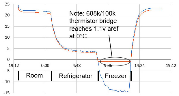
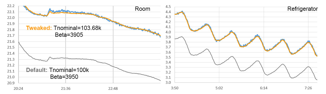
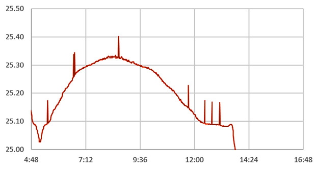
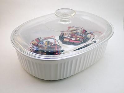
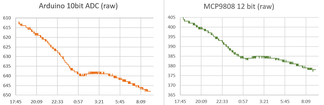
Thermistors are really twitchy due to their low thermal mass, so I did this test inside of a large ceramic pot with a lid to smooth out the changes.  At first bounce I though that jitter on the thermistor line was due to poor resolution, but it turned out to be an artifact of  the calculations I was doing in Excel.

When I compared the raw output of the Arduino ADC and the 9808:

Though the left axis is inverted for the thermistor, the scale on both is the same showing that the effective resolution is better than the 12-bit sensor. (click the image for a larger version)

Though the left axis is inverted for the thermistor, the scale on both is the same showing that the effective resolution is better than the 12-bit sensor. (click the image for a larger version)

So perhaps correcting the initial 3.3v VrefL offset reading with that Vcc ratio was not such a good idea, and I should avoid mixing different resolutions by taking a post 1.1v read of VrefL for offset correction.  Even if that is the case, tracking the positive rail still seems like a good idea for a data logger, so I will add it to the once per day events that get triggered by the 24 hour rollover.

So the job’s done with  four resistors and bog standard 10K NTC right?

Uh uhh… In fact this is just the stuff I had to get a grip on before starting my quest for the ADC holy grail.  I didn’t want something as good as the 12-bit sensors, I wanted something better, and the semi-mythical technique of oversampling promised to deliver all the resolution I could ever want from a humble Arduino… in theory

But this post is already miles too long, so for now I will just leave you with a teaser from a recent run-test showing output from an 24-bit MS5803 vs256 sample average using the Arduino ADC and that same 10k NTC thermistor:

Teaser_14bitditheredjpg

Y axis=temp in °C    Note: I have offset the curves here for easier visual comparison. The resolvable feature size is already well below 0.01°C and I am sure that I can push that a bit farther…

You have to throw in another resistor, and a couple of capacitors, and I still have some niggling details to work out optimizing the technique to use the least amount of power. When I get all that sorted, I will post the gritty details…

Addendum 2016-06-23:

There is a thermistor based Compost Sensor project by kinasmith at Instructables which uses wireless Moteinos and a cellular module to relay the data. Cool stuff.  Also there is a discussion of the lookup table method to address the accuracy of your thermistor readings (which I did not really talk about in this post) over at Mike’s Lab Notes.

Addendum 2016-08-01:

In this blog post, Ejo puts an ADS1115 / thermistor combination through its paces, using a combination of single and differential readings to remove voltage bias.  His resolution  reached 0.00427°C    And here is another group combining the ADS1115 with a bridge.

Addendum 2017-02-27:

Well it took a lot longer than I expected, but I finally got the post on How to do Oversampling with an Arduino out the door. The pin toggling method I’ve come up with is pretty darned easy, and gives you access to at least 4-5 more bits of ADC resolution.

Addendum 2017-04-26:

I’ve moved on to calibrating the thermistors, and in the process I learned that it’s probably not a good idea to combine the 1.1v aref, with the oversampling method. But I did it anyway.

Addendum 2017-09-26:

You could get another bit of hardware resolution with a two element varying bridge and then doing a Pseudo-Differential reading with the Arduino ADC.  I still haven’t wrapped my head around the math for that yet, which would get tricky if you were simultaneously using 1.1v aref – since your bridge could not be symmetrical.

Addendum 2019-03-25:

I’ve been developing a new method for reading thermistors with the Input Capture Unit on pin D8. Micro-controllers count time much more precisely than ADC’s measure voltage, so this new approach delivers more resolution than 16-bit oversampling in about 1/10th the time & power.

Field Report 2016-03-16: Rain Gauges Over Reporting

Fer_RioExchange

As this was a dry part of the cave, I even risked bringing in the laptop…

One of the first priorities was a trip out to Rio Secreto to service drip loggers. Data from the last season confirmed that all of the loggers are good for at least 6-8 months, so we now have the option of servicing some units, while leaving others for a later trip. As the install base continues to grow, that’s becoming an important consideration for the trip logistics. Even so, our schedule was pretty tight so we decided to try servicing the units ‘in-situ’, so we only had to make one trip.

The forest floor gauge was knocked over by critters, despite a fairly hefty anchor.

Mapaches?

After that I tackled the climate stations we had on the surface. I was keen to see data from the logging rain gauges as this was only their second real-world deployment.  Back in Dec. we deployed two units, with one on the roof of a building, above the tree canopy, and one on the forest floor. My heart sank when I found that something had knocked the forest unit over, despite a fairly hefty cement anchor. That happened only a couple of weeks before our retrieval, so we still had a fairly complete data set.

Our original thought was to use the comparison data to see how much rainfall was being intercepted by the canopy, but the sheltered forest floor record also ended up providing me with some vital information about how wind was affecting the rooftop unit:

F

TypicalDailyWindNoise

The ground unit had none of these 0-15 count spikes which peaked at mid-day (local time).

The drip counter inside the rain gauge is essentially using it’s accelerometer as a vibration sensor, which gave us in-cave sensitivity down 12cm drip-fall distances. So it probably should have occurred to me that we needed to reduce the sensitivity for surface applications.  The daily noise is pretty easy to threshold away in Excel with an if statement [ =IF(DataCell-threshold<0,0,DataCell-threshold) ] and different settings showed that the typical daily ‘background noise’ was adding about 10%.  I’ve even heard that funnel wetting & other losses cause cheap rain gauges to under-report by that much, so this daily bump might come out in the wash.  A thornier problem lies with the ‘windy day’ events, which produce the larger spikes. And that effect is probably embedded in the rain storm data as well.  Though with ~10 drops counted per mL of water through our funnel,  actual rain events usually count up into the thousands.  So I can apply pretty aggressive filtering (with thresholds around 200) and doing so hints that the stronger wind events are probably adding another 20% to the overall totals. I know that’s sounds pretty bad, but hey – it’s a prototype right?

So there are a batch of sensitivity trials ahead, and once again I need some external data to calibrate against.   Of course anything that can count accelerometer alarms can just as easily be counting reed switch closures, so it’s back to the bench I go… 🙂


Spotted in Tulum:

Signal2Noise

Signal-to-noise ratios…

<— Click here to continue reading the story—>

Field Report 2015-12-08: The DIY Logging Rain Gauges Work!

Trish & Fernanda inspecting units before retrieval

Trish & Fernanda inspecting units before retrieval

We managed to squeeze in a short  fieldwork trip before the end of the year, and the growing number of loggers at Rio Secreto put that cave at the top of our list to give me enough time to service all the units.  It was also important that we get everything back into place before they were swamped by tourists wanting to spend their holidays in the sun, rather than shoveling snow.

I was very happy to see that only one single machine suffered a sensor failure, and this was one the surface drip units that we had cooked under the tropical sun during a previous deployment.  Some of our early monitoring stations are finally passing that critical one-year mark, so we can start to think about seasonal patterns in records that display this kind of short term variability:

Typical Drip Sensor record 2015, Rio Secreto cave

Drip count /15 min,  Station 10, Far Pool Cluster

RainGauge

I had no idea spiders were so fond of  living in climate stations…

We also had a several sensors on the surface, and I was really curious to see the the data from this first field deployment of the new rain gauges, given that so many of our cave records showed strong discontinuity events like the one above.  Not only did I want to see the quantitative data, I also wanted to know if the bottom shroud prevented the internal temperatures from going into to the 60°C range (which damaged several earlier loggers…)

And…. success! And both rain gauges were within 5% of each other, despite accumulations of bird poop & leaf litter, and one unit suffering from a slow tilt of nearly 10 degrees as the palapa roof shifted underneath it. With conversion ratios from my back-yard calibration, we were able to translate the drip counts directly into rain fall:

Rainfall (cm/day) data from one of our first rain gauge prototypes at rio Secreto

Rainfall (cm/day) from one of our first rain gauge prototypes at Rio Secreto

Trish had her doubts about this record initially, with so much rainfall occurring in what was supposed to be the local ‘dry’ season.  But after searching through data from nearby government weather stations, and comparing our surface record to the break-through events I was seeing in the drip data, we slowly became convinced that it had, in fact, been one of the rainiest dry seasons in quite a while.  We also had a beautiful temp record that showed the new cowlings pulled peak temperatures (inside the loggers) down by almost 20°C:

Rain gauge internal Temp from RTC registers.

Rain Gauge, Internal Temp (°C) from the DS3231 RTC register.

Hopefully this means that the SD cards are back in the safe operating zone, which I know from past failures is nowhere near the 85°C that Sandisk claims.

So the new rain gauges are working properly, adding another piece of hydrology instrumentation to the Cave Pearl lineup.  I would love to say that the Masons Hygrometers delivered another great success, but the analysis is turning out to be somewhat more complicated as the 96-98% RH variations pulled my wet bulb depressions right into the bit depth limit of the DS18b20’s , so I will have to keep you in suspense for a while as I chew on those numbers…

Addendum 2016-03-16

Well serves me right for counting my chickens: Turns out that the drip sensor based rain gauges suffer from spurious counts due to wind noise. But I’ve been running these guys at their highest sensitivity settings, so hopefully I can dial that back to reduce the problem. We also had the gauges on a soft palapa roof, which no doubt contributed to the problem.

<— Click here to continue reading the story—>

Measuring Humidity with Arduino: A Masons Hyrgometer Experiment

The housings could be much smaller than this, but I wanted

The next generation of flow sensors running “hang” tests so I can quantify sensor mounting offsets. I like to see a few weeks of operation before I call a unit ready to deploy. Each new batch suffers some infant mortality after running for a few days.

I’m finally getting the next generation of Pearls together for their pre-deployment test runs. The new underwater units will all be in 2″ enclosures and perhaps it’s just me, but I think the slimmer housings make them look more like professional kit. These units are larger than I would have liked, but with six AA batteries they needed some extra air space to achieve neutral buoyancy. With the slow but steady improvements to the power consumption, this might be the last batch designed to carry that much juice.  There are a host of other little tweeks including new accelerometers because despite all the hard work it took to get them going the BMA180’s did not deliver the data quality I was hoping for. It would seem that just having a 14bit ADC does not always mean that the sensor will make good use of it. This is the first generation of flow sensors that will be fully calibrated before they go into the field. That’s important because most of these guys will be deployed in deeper saline systems with flows slower than 1 m/s.

The newest Cave Pearl is a Masons hygrometer that will use DS18B20 sensors for the wet & dry bulb measurements

This is a sensor cap for the Masons hygrometer experiment which uses waterproof DS18B20s for the wet & dry bulb readings, with the extra sensor letting me compare different drip sources simultaneously. An MS5803-05 records barometric pressure, and I put a (redundant) MCP9808 in the leftover sensor well to track the housing temperature.

A new crop of drip sensors is ready, and this time a couple of them will be based on the Moteino Mega, with a 1284 mcu providing lots of SRAM for buffering.  They performed reasonably well on bench tests but it will be interesting to see how they fare in the real cave environment. The drip loggers we left on the surface as crude rain gauges will be upgraded with protective housings and catchment funnels, hopefully providing a more accurate precipitation record. They will be joined at the surface by new pressure/temp/r.h. loggers that sport some DIY radiation shields and they will have none of the Qsil silicone which swamped out the barometric readings with thermal expansion last time.

I use a shoelace as a wick to cover the wet bulb.

A bit of shoelace becomes a wick for the wet bulb. It’s made from a synthetic material, as I suspect that the traditional cotton wicks would quickly rot in the cave.

And we will have a couple of new humidity sensors to deploy on the next fieldwork trip. The rapid demise of our HTU21D’s back in December prompted me to look for other methods that would survive long periods in a condensing environment. That search lead me to some old school Masons hygrometers, which in theory let you derive relative humidity with two thermometers provided you keep one of them wet all the time so that it is cooled by evaporation. The key insight here is that I am already tracking drip rates, so I have a readily available source of water to maintain the “wet bulb” for very long periods of time.  If the drip count falls too low I will know that my water source has dried up, so I will ignore the readings from those times.

Underwater deployments have already proven that the MS5803 pressure sensors are up to the task and waterproof DS18B20s look like they might have enough precision for the job.  The relatively poor ±0.5°C accuracy of the DS18’s does not matter so much in this case as the “wet bulb depression” is purely a relative measurement, so all you have to do is normalize the sensors to each other before deploying them. I still had a few closely matched sets left over from the temperature string calibrations, so I just used those.

Hopefully this SHT-11 sensor from Seed studios will run a bit longer than the HTU21's that died so quickly last time.

This RH sensor has a copper sintered mesh, and all the non-sensing internals are coated with silicone. It’s worth noting that the SHT series does not play well with I2C sensors, and must have it’s own set of dedicated com pins. It also pulls far more current than the datasheet says it should, so this logger draws a whopping 0.8mA while sleeping. I’m driving it with the library from practical arduino’s github, so perhaps something in there is preventing the SHT11 from sleeping(?)

Of course there are a host of things that I will be blatantly disregarding in this experiment. For starters you are only supposed to use pure distilled water, and cave drip water is generally saturated by its passage through the limestone. Perhaps the biggest unknown will be the psychrometric constant, which changes pretty dramatically depending on ventilation, and with several other physical parameters of the instrument. Since there is no way I am going to derive any of that from first principles, I though I would try a parallel deployment with a second humidity sensor so I could determine the constant empirically. The toughest looking electronic R.H. sensor I could find for this co-deployment was the soil moisture sensor from Seeed Studios. Even with it’s robust packaging, I expect it to croak after a few months in the cave, but hopefully the SHT11 will give me enough data to interpret the readings from the other hygrometer.

Once the epoxy had cured, I set the two units up in the furnace room so the wet bulb was not ventilated. Recent heavy rains meant our basement was hitting 75% RH, and I had a dehumidifier running at night to pull that down to 55%. (far from the Masons so there was no air movement at the wick!). That test produced wet-bulb depressions between 2-4 degrees Celsius, allowing me to create the following graph:

FirstMasonsTestRun

Even with the psychrometer constant bumped up to 0.0015  (0.0012 is usually quoted for non ventilated designs with warnings that the number will be different for each instrument) the Mason is reading about 10-12% above the SHT11.  I can deal with that if the offset is constant, but it means that the difference between the two bulbs is smaller than it should be. That is typically the direction of errors for this kind of design but when the humidity gets up into the 90’s, my humble DS18’s might not have enough resolution to discriminate those small differences – especially if there is some ugly non-linear compression happening.  You can already see some of that digital grit showing up on the green plot above. I was pleasantly surprised to see very little difference in the response time for the two sensors, although I suspect that is because they both have significant lag. 

For a first run, those curves match well enough that the method is worth investigating. We can put up with lower resolution & a lot of post processing if the sensor will operate reliably in the cave environment for a year.  And if the idea doesn’t work I will still be left with a multi-head temperature probe, which can be put to other good uses. I will build a couple more of these, and keep at least one at home for further calibration testing.

Addendum 2015-07-21

The closest thing I have to a cave environment is an enclosed space under the porch.

I did not use distilled water in those reservoirs, as the cave drip water will have plenty of dissolved solutes which will shrink the wet bulb depressions

I set up the new hygrometer caps for a long run in an enclosed storage space under the porch; which is the closest thing I have to an unventilated cave environment. Fortunately the weather obliged with a good bit of rain during the test, pushing the relative humidity up towards the 90’s where the loggers will be spending most of their time after they are deployed. These builds include pressure sensors, but the one I will be keeping at home also has an HTU21D R.H. sensor, since the SHT-11 I am using as my primary reference will go into the field.

Readings from the HTU21 vary between 4-6% lower than the SHT-11:

HTU21dvsSHT

So as usual, having multiple sensors to read RH directly puts me back into “the man with two watches” territory; though I have slightly more faith in the Sensirion.  If I match the overall dynamic range of the Mason output to the soil moisture sensor by tweaking psychometric constants, I can bring the them within 3.5% of the SHT (with uncorrected R-squares > 0.93) :

RH 3 units compared

I was hoping that those psychometric constants would be much closer to each other and I will have to chew on these results to see if I can figure out what is causing the variance between the instruments. I would also like to know where that positive 3.5% offset comes from.

I should mention here that a similar offset problem affects the atmospheric pressure sensors which I need to calculate the actual water vapor pressure using:

Saturation Vapor Pressure @ wet bulb temp:
= 0.61078*EXP((17.08085*T(wet))/(237.175+T(wet)))
Actual Vapor Pressure:
= Sat. V.P.@wet bulb – [ (psy. constant) (Atm.Pressure in kPa(T(dry)-T(wet)) ]
Relative Humidity:
= (Actual V.P./ Saturation V.P.)*100

Fortunately at weather.gov they post three days of historical data from your local NOAA weather station, which you can use to find the offset for your home built pressure sensors:

FindingPressureSensorOffset(Note:I had to concatenate the date/time info into Excel’s time format to make this graph)

Most of my MS58xx sensors seem to have a -10 to -20 mBar offset after they are mounted. I suspect that this is due to the epoxy placing strain on the housing because of some shrinkage while curing. Overall variations in air pressure have a small effect on the calculation, and many wall mount hygrometers don’t even specify corrections for elevation. So you could probably use this method reasonably well without a “local” barometric sensor by just putting 101.3 kPa in the calculation.

Addendum 2015-07-22

I just stumbled across a neat soil moisture sensor project, that measures moisture dependent conductivity through some Plaster of Paris in a straw. I’m not sure it would give me the durability I need for long cave deployments but it still looks like a great DIY solution. It would be interesting to see how they compare to the commercial gypsum based sensors which usually run around $40 each.

There’s also a good overview of calibrating RH sensors with saturated salt solutions  by Samantha Alderson and Rachael Perkins over at A.M Art Conservation,

Addendum 2015-07-23

A helpful comment over at the Arduino.cc sensors forum put me onto this tutorial. I did not know that the meat & dairy industry is still using wet & dry bulbs to monitor R.H. so I have a new place to look for information on the method. There is another document over at Sensors Magazine at Sensors Magazine outlining how a thermistor pair can be used to determine humidity if one is hermetically encapsulated in dry nitrogen and the other is exposed to the environment. You drive current through the sensors to produce self heating, and then measure the differential cooling rates of the dry nitrogen vs exposed sensor to derive the humidity.

Addendum 2015-08-14

Two Masons Hygrometers are now deployed in Rio Secreto cave next to my drip loggers:
(I will keep the third one at home for further testing) 

With two dry bulb probes suspended in air, while wet bulb is fed by the drip station.

This unit has the two dry bulb probes suspended in air with cable ties, while the wet bulb is fed by runoff from a drip station. I tried to choose a station that does not run dry at any time through the year.

It will be at least four months before we pull these units and find out if the experiment worked. Fingers crossed!