
So far in 2024 we’ve released DIY calibration procedures for light, pressure & NTC temperature sensors that can be done without expensive reference equipment. Important techniques; but with long environmental time-series the 500 pound gorilla in the room is actually time itself. Precise timekeeping is something of a back-burner issue in the hobbyist world because so few are trying to combine data from multi-sensor arrays. And syncing to an NTP server is easy when you are already using wireless coms – provided that’s ‘good enough’ for your application. However for people who want high accuracy, using NTP is like setting your watch by constantly asking a friend what time it is.
Reconstructing a sequence of events in a dynamic earth system is challenging when timestamps are generated by independent and unsynchronized clocks. But our loggers get deployed by the dozen in underwater caves, and even when you are above ground wireless isn’t really a long term option on a single Cr2032. For stand-alone operation we rely on the DS3231 RTC as they usually drift about 30 seconds per year – but there are always a few outliers in each batch that exceed the datasheet spec of about 5 seconds per month (±2ppm) for the -SN and 13 sec/m (±5ppm) for -M (MEMS) chips. These outliers are hard to spot with our usual ‘by hand’ time-setting process over the serial monitor. You can get a set of loggers within 80 milliseconds of each other with that method, but that difference is still annoyingly visible when the LEDs pip. That set me hunting for a better solution.
Paul Stofregens TimeSerial is often suggested but TimeLib.h didn’t play well with the RTC functions already in our code base. Even after sorting that out, and installing Processing to run SyncArduinoClock, I was still initiating the process. So TimeSerial didn’t get me any closer to the perfectly synchronized LEDs I was after.
SergeBre’s SynchroTime seemed like an all-in-one solution. But even after a decade working with the Arduino IDE, I still made every newbie mistake possible trying to compile that C code for windows. There are simply too many possible editor/ compiler/ plugin combinations to sift through without a lot of mistaken installations, removals & re-installs. I wasted a couple of days before realizing that code was packaged for the QT environment, and when I saw the additional cost I finally had enough. In the end, it took me less time to build my own GPS time-sync code than I spent trying to compile SynchroTime. That’s an important lesson in the difference between something that’s technically open source and a useable solution. Of course I can’t write that without wondering how many feel the same way about this project.
Jump links to the sections of this post:
- Step 1: Determine the Optimum Aging Offset
- Step 2: Synchronize RTC time with a Neo6M GPS
- Step 3: Testing and Verifying Clock Drift
- Last Word
- References & Links
Step 1: Determine the Optimum Aging Offset
Despite those setbacks, I couldn’t give up this quest knowing that HeyPete had achieved a drift of only 26 seconds with DS3231 offline for 3 years. The key to that spectacular result was tuning the Aging Offset Register before the run. Positive values in this register add capacitance to an array, slowing the oscillator frequency while negative values remove capacitance and increase the main oscillator frequency. The change is different at different temperatures but at 25°C, one LSB adjusts by approximately 0.1ppm(SN) or 0.12ppm(M). The exact sensitivity is also affected by voltage and age so it can only be determined for a given chip empirically. The datasheets also warn not to run noisy PCB traces under the RTC that might induce capacitive/coupling effects on the crystal but many modules on the market ignore this. My ‘rule of thumb’ when servicing loggers in the field is that changing the aging register by ±3 will correct approximately 1 second of clock drift per month when I don’t have access to the resources described in this post. Of course that requires you to have good field notes so you can be sure when the logger’s clock was last set.
In April 2023, ShermanP proposed a method to do this using successive approximations via the Arduino system clock. After considering, and then rejecting, NTP & WWVB, he settled on GPS as the best source and then posted a ready-to-run solution on his GitHub repo: https://github.com/gbhug5a/DS3231-Aging-GPS
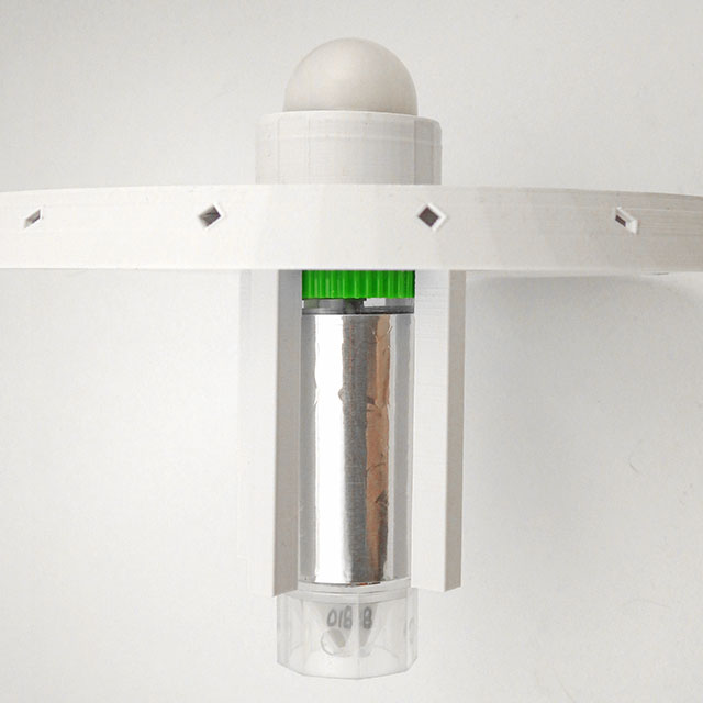
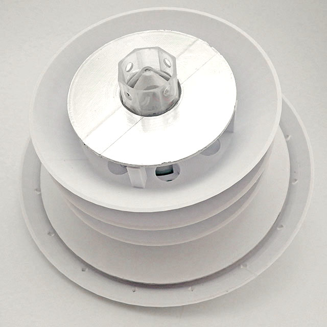
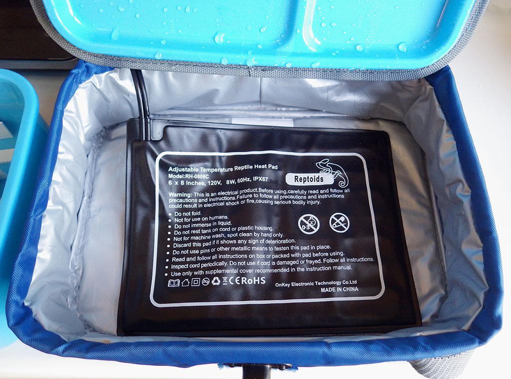
Before proceeding further, read the PDF to understand how his code works. The key idea is that “In calibrating the optimum Aging setting, you should duplicate as nearly as possible the power supply voltage the RTC will experience in its application.” although I suspect this is less critical for the crystal based -SN chips than for the MEMS oscillators. Unfortunately battery voltages change significantly with temp. so matching the rail implies you are also doing this RTC adjustment at temps near your expected deployment ranges – which may not be possible. The Cr2032s that power our loggers spend most of their operating life at 3.05v, and the power indicator LED on raw RTC modules pulls enough current that it drops the UNO’s 3.3 volt line down to about 3v. Finished loggers draw only 1-2μA while sleeping so for those I have to add a Schottky 1N5817 inline to drop that supply down to 3.05v during the test.
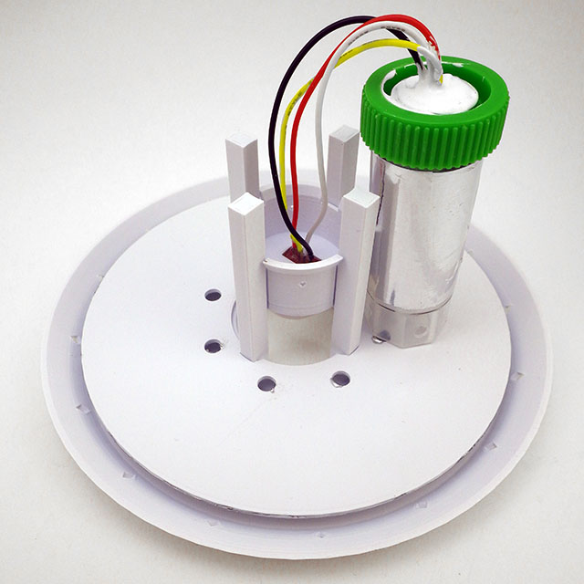
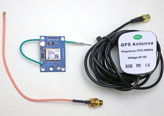
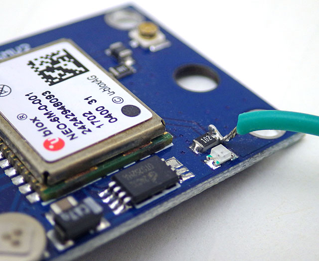
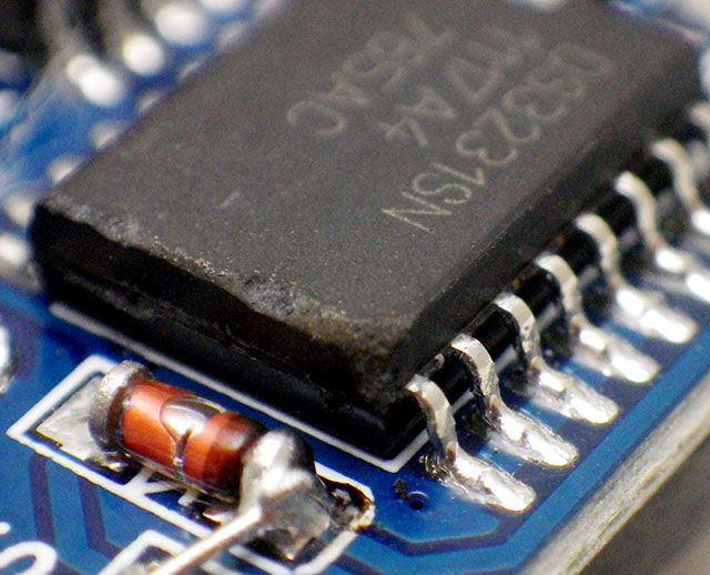
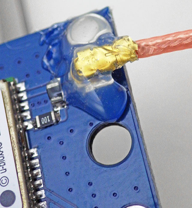
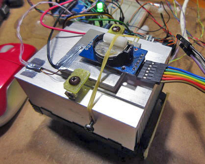
[this photo shows the GPS PPS connected to D3]
Sherman’s code uses the Interrupt Capture Unit so the PPS signal from the GPS must be connected to D8. I put a male Dupont pin on the end of the PPS tap so the UNO connection can be moved easily as the other code in this post requires that connected to D3. When testing the RTC inside assembled loggers, I have to use an alligator clip ( in green above ) for the alarm line which already has a soldered wire connection – so a female Dupont will not fit over that header pin.
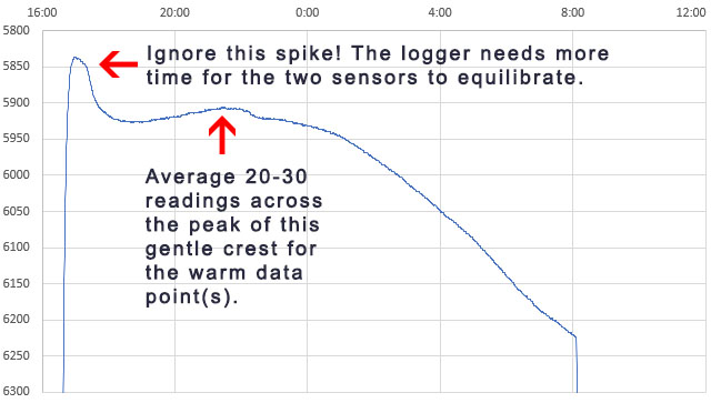
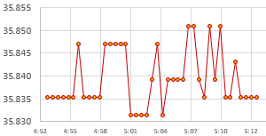
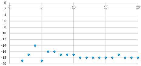
It usually takes 20-30 minutes for the adjustment on a -SN chip to reach a stable value, or settle into a pattern toggling the last bit up and down:
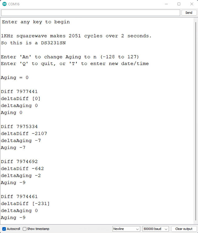
Unfortunately the DS3231 has no non volatile memory which means all registers will reset whenever the chip loses power. So I write the optimum offset from this test on the modules battery holder with a white paint marker during the component triage I do before building new loggers. Most of the time I get similar results when running this test on a completed build that I got from the RTC module by itself before the logger was assembled. However for about 1/3 of the RTCs, forcing the chip to run in low-power mode from Vbat slows the main oscillator speed up to 2ppm – so the only safe approach is to retest the age register test after logger assembly. The BBSQW battery power alarm enable (bit 6 of the 0x0E register) must be set when running the RTC on Vbat.
SN chips settle to a stable offset value quickly: usually within 2-3 cycles but it can take an hour or more before the -M chips give you a stable age offset. About one in 40 of the RTC modules does not settle to a consistent number no matter how long you leave it and I toss those as defective. Occasionally this is because even with the Age register pushed all the way to a max value (±127) the RTC still can not match the GPS pulse. Some of the non-calibratable units have a non functional register – you can write a value to the register and read it back but that has no effect on the output. I suspect that many of these failures are due impact damage after the chip has been dropped. I also reject any RTC where the temperature register is off by more than 3°C because they won’t be able to do the TCXO corrections. The aging register and the temperature adjustments get combined at the load capacitor bank to tweak the main oscillator, so aging register changes won’t get applied until the next (64 sec) temperature correction unless you also trigger a manual conversion. Just by chance, about one in 25 of the -SN chips keeps almost perfect time compared to the GPS with the register left at the zero default. For now I’m keeping those aside as secondary reference units.
To leave room for a decent range of TCXO correction, and with ±2ppm short-term wander (on the Mems chips) the aging register should only be used to compensate for about 6-7 ppm of baseline offset. I try not to use a module where the aging register correction to match the GPS is more than ±50.
Step 2: Synchronize RTC time with a Neo6M GPS
Most clock projects use NTP, but there are a few that go that extra mile and synchronize to GPS. One that caught my attention was: Super-Accurate GPS-Corrected RTC Clock – without Internet NTP He avoided the serial bus latency of those pokey 9600 baud coms by preloading variables with GPS time +1second and then waiting for the next GPS pulse before setting the RTC registers. With this concept in hand, and TinyGPS++ to parse the NMEA strings, it didn’t take long to whip up my own version for our loggers. It’s worth noting that several forums mentioned NMEA messages can exceed the 64byte buffer in SoftwareSerial so I increased this to 128 bytes by editing the file at: C:\Program Files (x86) \Arduino \hardware \arduino \avr \libraries \SoftwareSerial \src
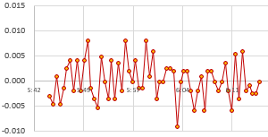
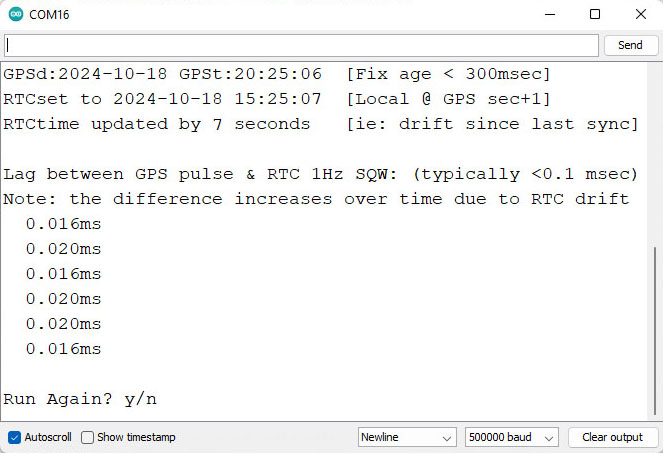
Another hidden gotcha is that GPS time can be out by 2 or 3 seconds until it receives a ‘leap seconds’ update which is sent with the Almanac every 12.5 minutes. So wait until the sync LED has been blinking for 15 minutes before setting your clock time as I don’t (yet) have an error catch for this. Our RTC time-sync code displays how much adjustment was done to the RTC time and checks the latency between the GPS pulse and the new RTC time immediately after the sync. That difference is often less than 30 microseconds, but it increases from there if you leave the system running:
You still have to edit the code by hand for your specific local-time adjustment but everything is well commented. Most scientists run their loggers on UTC which matches GPS default time so that local time tweak can be commented out.
One small issue with having to run these test utilities with the RTC at 3.05v is that you’ll need to change the battery before deploying the logger. To preserve the clock time, connect the logger to a UART so the RTC is powered continuously during any battery swaps. After the time-sync & new battery, the normal procedure is to load a logger with its deployment code which has a start menu option to set the RTCs aging offset. This gets saved into the 1k EEprom on 328p processor and once set, the base-code automatically reloads that value from the EE into the RTC’s aging register at each runtime startup. After that’s done the logger is ready to deploy – so Step 3 below is only for those who want to explore the DS3231 RTCs drift behavior in more detail.
Step 3: Testing and Verifying Clock Drift
Now that we have the aging offset, and the RTC is synced to GPS time, how do we verify what we’ve done?
One method is simply to run the clocks until the drift can be easily measured – but that can take several months. You can get immediate results by enabling the 32kHz output on a DS3231-SN and comparing that to a high accuracy source with an oscilloscope. Ideally, you calibrate to a traceable standard which is at least one decimal place better than your device resolution. Kerry Wong did this with an HP 5350B Microwave Counter and HeyPete uses a Trimble ThunderBolt Timing GPS. There are a few retired engineers out there with universal counters on the bench and for truly dedicated ‘time-nuts‘ only an atomic clock will do. But even then the times from several must be averaged to arrive at a published value, and whenever you achieve better numbers by averaging multiple measurements you obscure potential issues with jitter.
Even if we had that equipment budget, our loggers supply the DS3231 from Vbat to save runtime power which disables the 32kHz. And -M chips don’t support that temp. compensated output no matter how they are powered. So is there any validation test that can be done without expensive kit or the 32khz line?
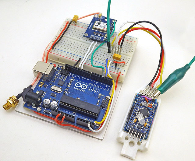
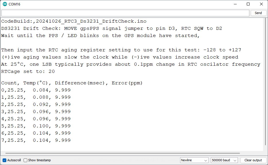
Actually there is – thanks to the Needle Nose Pliers blog in Tokyo. He developed a method that uses least squares over one minute of aggregated readings to resolve rates of change below 0.02μs/second despite the fact that an UNO sysclock only ticks at 4μs. I wrapped his calcSlope() function with modifications needed for the UNO/NEO6 test rig used here and added an input to change the Aging register before each run. To run the drift checking code from our Github, connect the GPS PPS to D3, and RTC SQW to D2:
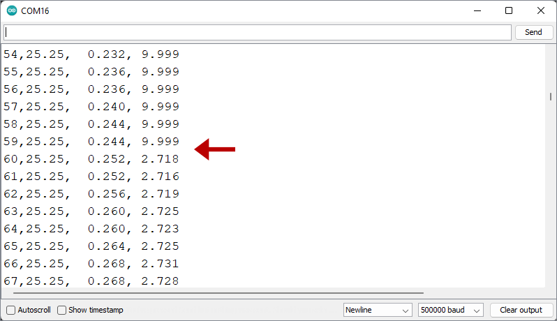
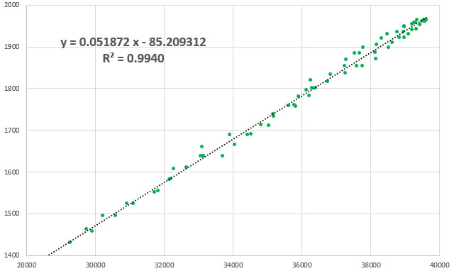
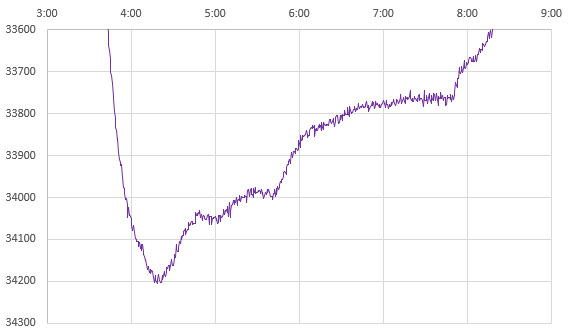
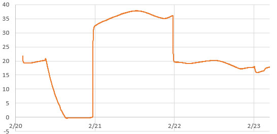
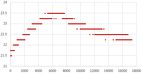
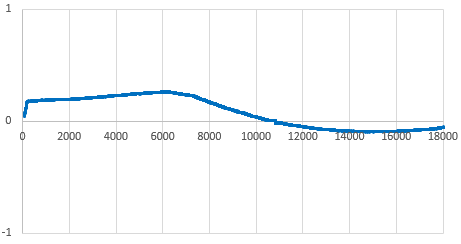
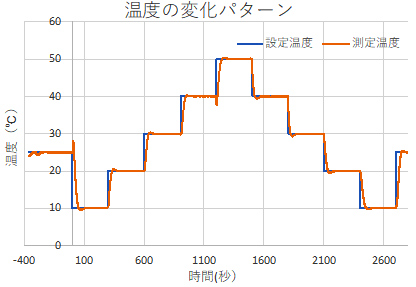
That serial output can then be copied into a spreadsheet to compare the effect that different aging offsets have on the RTC. Here are the results from two five-hour tests of a DS3231-M; first with the the Age register set at zero and then with it set to -17. The clock time was sync’d to GPS time before each test to make the graphs easier to compare with the x axis is seconds: (click to enlarge)
RTC temp. during test —> Msec offset from GPS —> Drift Error PPM
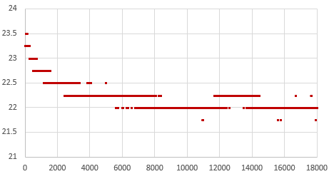
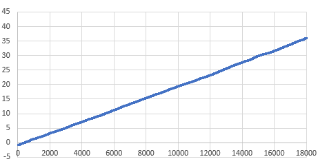
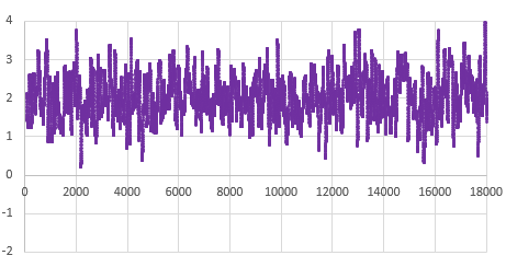
At the Age=0 default, this RTC’s 1Hz output was 35 milliseconds behind the GPS pulse after five hours, which would be roughly equivalent to 100 seconds of drift per year. The average error hovered around +2 ppm. This is well within spec for a -M chip as ±5ppm implies up to 155 seconds of drift per year.
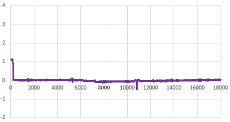
Then the Aging register was set to -17 (as determined by the test from Step1) and the drift examination was done again. That same RTC module was now only 0.5 milliseconds behind the GPS pulse after five hours, with the slope-derived error averaging close to zero ppm:
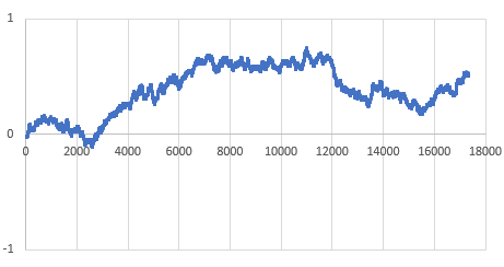
So with the correct aging offset this -M chip could be expected drift less than a second per year. Of course this only applies near our Step1 testing temperature, but in general: If you found the best aging offset correction, the msec difference between a 1Hz alarm from the RTC and the GPS pulse should change very little over a short test.
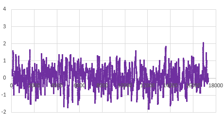
Its worth noting there is ±2ppm of jitter in the calculation with that -M chip (above) that is not present for -SN chips. The -SN shown below had a straight linear drift of 20 milliseconds slow over five hours when its Aging register was left at the zero default (that’s about 35 seconds/year or 1ppm), but the same RTC had near zero milliseconds of drift over five hours when the aging offset was set to -21:
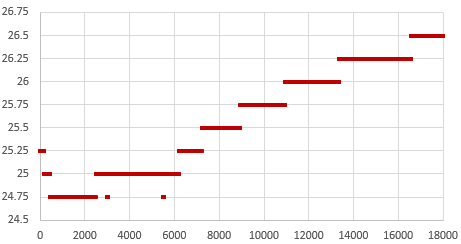
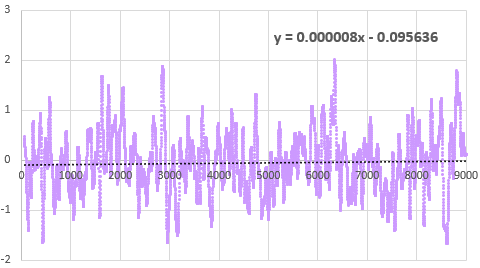
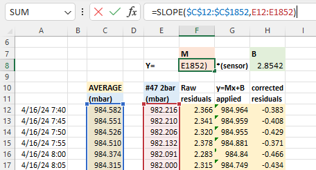
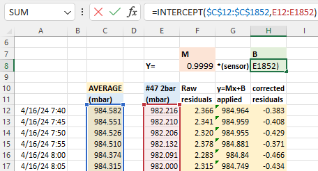
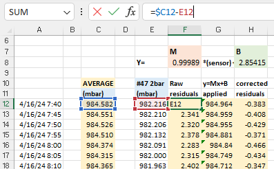
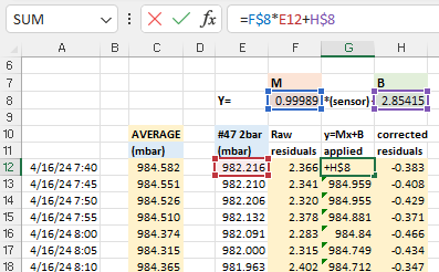
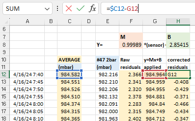
Even with temperature rising 3°C during the test, that -SN stays within a tighter tolerance than the -M. This difference in short-term variability explains why the offset determination settles so quickly with a -SN, but can wander around for some time with a -M. The code used here in Step3 is like a slow verbose version of what’s being done in step1 that shows all the intermediate readings. If you put a linear trendline on the graph of the error PPM from running this test with the offset left at the zero default, you can estimate how much age register adjustment it would take to shift those readings until the average is near zero. The aging offset suggested by the test in Step1 should be close to the result of dividing the ‘b’ term from the y=mx+b trendline fit equation by 0.1ppm(SN) or 0.12ppm(M), and changing the sign.
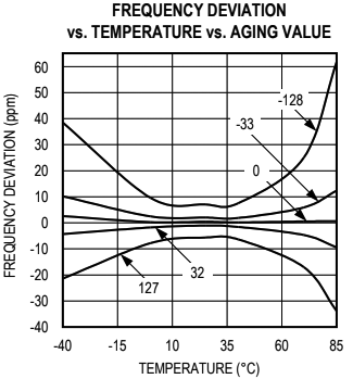
On his blog, NNP also demonstrated how the two chip variants have different responses to temperature changes:
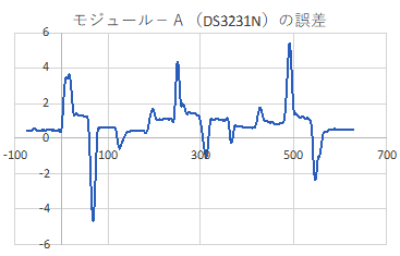
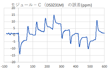
[ images from: http://radiopench.blog96.fc2.com/blog-entry-960.html ]
This confirms what I already suspected from our data: the -SN chips are a much better choice for outdoor environments where temperatures vary over that entire 50°C range. Although the temperature coefficient of the MEMS oscillator is not specified in the datasheet, loggers built with -M chips are probably still fine for stable thermal environments and with a tuned Aging register I’d expect them to drift less than ten seconds per year indoors. There are other insights if you dig into NNP’s blog. For example, drift is also affected by the physical orientation of the chip with respect to gravity. I had no idea it was a problem for all quartz resonators unless the crystal is cut into a special shape to avoid it. This highlights the fact that with so many different factors affecting the RTC, the Aging offset adjustment will never be perfect; you are simply aiming to reduce the ‘average’ drift. These tests are also affected somewhat by the stability of the oscillator on the UNO so we have a chicken & egg thing there.
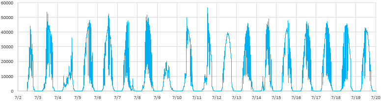
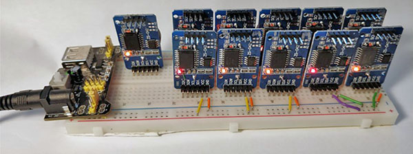
I will be doing more tests to see what other insights it can give into our ProMini / DS3231 combination. With the ability to synchronize clocks so precisely (in Step 2) you can see the outliers in a group in as little as 24 hours simply by watching the LED blinks. I already do multiple rapid burn-in tests with new loggers as part of pre-deployment testing, so visually checking synchronization during those runs is low-effort way to verify the RTC. One thing I’ve long suspected, but have never seen any actual proof of, is that the process of updating registers and generating alarms also affects the clock time. Perhaps handling the I2C transaction blocks the update of some internal counter? I could test this by setting one logger in a ‘well matched’ group to wake every second, while the others blink at five seconds, and see how many days it takes for the fast blinker to shift out of alignment.
It would be interesting to get a couple of the newer DS3232 / DS3234 chips, and test how much they drift with their TXCO pushed out to 512 seconds for 1µA current, instead of the 64 second default that pushes the DS3231’s up to about 3µA average standby current.
Last Word
With these three tools to wrangle our time series we could see drift as low as five seconds per year from an SN in a stable environment, so our little 328p loggers can finally go toe-to-toe with all those smugly networked ESP32s. I will eventually combine these into a general RTC testing utility, but there are plenty of use cases for each as an isolated step – especially if you were tweaking the code for use with different RTC chips. Likewise, with the Neo being a 3v device I could add a few header pins to our loggers for the serial coms and run everything with the logger alone.
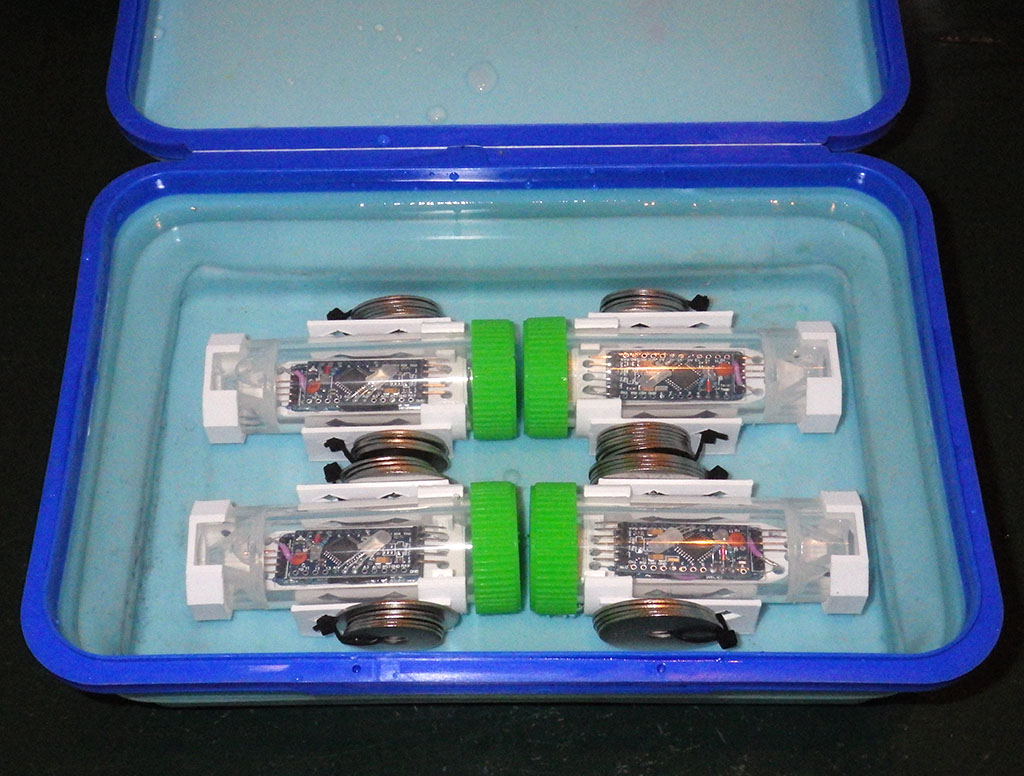
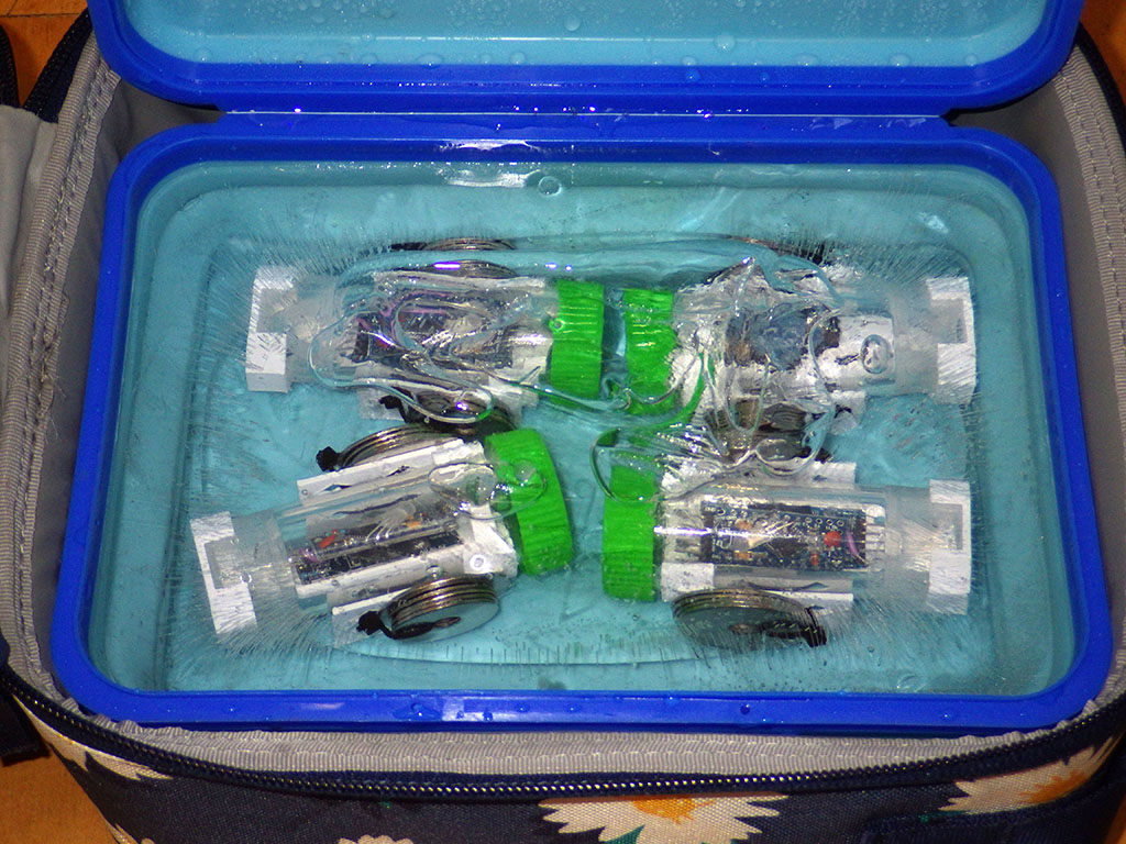
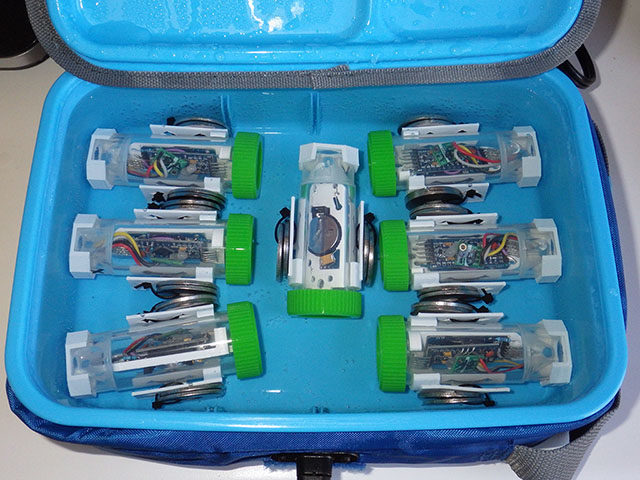
But I’m somewhat sentimental about the original UNOs, so it’s nice to dust them off once and a while. Another factor is that if you run two separate instances of the IDE you can choose a different com ports for each instance. So you can simultaneously have that UNO/GPS combination connected, and a ProMini logger connected via its own UART module. As long as you align the code open in each instance with the appropriate port, you can run those RTC tests on the UNO in the background while you work in the other instance of the IDE. This will be very handy when servicing loggers in the field. I will secure those field calibration rigs with hot glue and make them more compact with a ‘sit-on-top’ protoshield.
The quid pro quo when adjusting the Aging register is that the reduced drift within the tuning temperature range comes at the cost of increasing non-linearity at more extreme temperatures. But the underwater/cave sites we deploy into are quite stable compared to surface conditions, so it’s probably worth the trade. Physical aging rates are not necessarily constant or linear, so I expect that that register will need some yearly adjustment. Of course, if a logger has been in service that long I can just check how many seconds it has drifted and then tweak the AGEreg the old fashioned way: changing the register by ±3 corrects approximately 1 second of clock drift per month. The first complete generation of fully sync’d & calibrated RTCs will get deployed this fall, so it will be a while before I can check how aging is changed by exposure to temperature variations. I’ll be happy if I can get -M’s below 1 second of drift per month in real world conditions. I would hope to see the aging stabilize after the first year of operation in a manner similar to sensor aging.
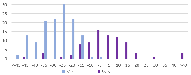
At the very least, we’ve greatly enhanced our ability to remove any real duffers from those cheap eBay parts. I’m still wondering what new sensor possibilities better time discipline might enable but I can already see some interesting labs for the next cohort of e360 students. One of the more challenging things to demonstrate within the constraints of a classroom is the relationship between datasheet error specifications and sensor drift. I’ll set aside a few of the worst -M modules for those teaching loggers so the results are more dramatic.
References & Links
Using a $1 DS3231 Real-time Clock Module with Arduino
A look inside the DS3231 real-time clock by HeyPete
5 Month DS3231 Drift Results at HeyPete.com
Setting the DS3231 Aging register to an optimum value by SermanP
Super-Accurate GPS-Corrected RTC Clock without NTP
Precise measurement of RTC error using GPS from Needle Nose Pliers
How they test Aging Performance in Crystals from Connor Winfield
Choosing the right RTC at Hackaday & module photos at Craft Corner
Comparing DS3231 / PCF8563 / MCP79400 / DS1307 RTCs
A collection of very detailed RTC tests from Dan Drown
And his GPS module measurements Part1, Part2, Part3 and More
An architect’s guide to GPS data formats, Estimating GPS time to FIRST fix
The U-centre program from u-blox, with multiple displays
Can the 60Hz mains frequency be used as a reference?
A Timing-sync Protocol for Sensor Networks
PTP clock synchronization over a WAN backbone
Arduino system clock accuracy [ ±1000ppm], various crystal error specs
RTC seconds/day to ppm drift calculator
Just adding a reminder here: the DS3231 doesn’t have a built-in mechanism to disable alarms after they’ve been set. You can clear the alarm flag to release SQW after it fires, but the alarm will still be armed and will fire again at the next time match – no matter how you set the alarm ‘enable/disable’ bits. The ONLY way to disable alarms on the DS3231 is to load those registers with an ‘invalid’ h/m/s combination that the actual time can never reach (eg: one with minutes/seconds set to 62 or, date set to Feb 31st). You can also set the EOSC bit of the control register to logic 1 which stops the oscillator when the DS3231 is on VBAT – but you will then be unable to check the clock drift at the next download. Halting the internal oscillator is the only way to stop the temperature conversions.
From the data sheets you can see that the -M uses half as much power (about 26 milliAmpSeconds/day) as the -SN chip does (45 mAs/d) to do its TXCO corrections however our standard Promini/DS3231-SN module combination usually sleeps around 890nA while the same logger built with a DS3231-M will sleep closer to 1680nA (when a temp compensation reading is not occurring). A sleeping 328p based ProMini draws ~150nA (reg removed & BOD off) and the 4K AT24c32 EEproms on the modules draw less than 50nA when not being accessed. So the -M chips that I’ve looked at seem to have more than 2x the ~700nA Ibat timekeeping draw of -SN chips. So they end up about the same in terms of total power consumed although the SN’s are still preferred because of their better drift/TXCO behavior overall.
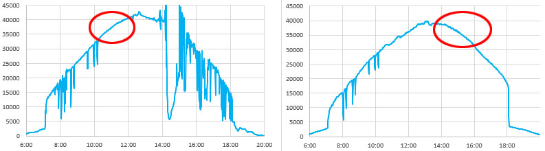
And lately I’ve been seeing a fault in these RTC modules that only shows up when you start to check the sleep current accurately: SN’s that do their TXCO corrections more frequently than the expected 64 seconds: often around 20-30 seconds. Other behaviors like temperature & time keeping seems fine. Measuring the current with a scope or CurrentRanger also makes it easy to spot when -M chips were deliberately relabeled as SN’s, because you see the temp correction spike every 10 seconds on the -M’s.