Field Report 2015-08-07: Retrieve Flow Sensor from Akumal Bay

Gabriel, Patricia Beddows, Marco A. Montes Sainz

Left to Right: Gabriel Sanchez Rivera / Patricia Beddows  / Marco A. Montes Sainz

I was up pretty late downloading the loggers from Rio Secreto the day before, so we had a late breakfast at Turtle Bay Bakery & Cafe the next morning. While the only decent coffee in Akumal has become something of a necessity for my aging brain, our corner table is also something of an office away from home for Trish, who knows so many people in the area that sometimes it’s hard to escape from all the hugs and hand-shakes.  With sufficient caffeine in my bloodstream I was ready to hit the reef with Marco, who had been keeping an eye on our little loggers through the Sargasso seaweed invasion that has affected coastlines throughout the Caribbean this year. He had already taken south bay unit out of the water due to a zip tie failure on the support rod.  I wondered if those dense floating mats had snagged the shallow unit, putting enough stress on the ties to break them?

Removing B4 from float line

Pulling B4 from it’s anchor rod.  (photo by Marco)

Since the B3 logger was already dry, that left only the Pearl at the north end of the bay. This B4 unit is the oldest continuously running logger on the project (it’s first underwater stint was back in March 2014) and is still running on it’s original Tinyduino core. Since the sensor is now well past my original one year design goal, I am tempted to retire it to the “bookshelf museum” as these old dogs feel like Russian tanks next to the new builds. But this project also embodies what the guys over at Boston Robotics distill down to “Build it, Break it, Fix it”, so I really want to see how long this DIY flow sensor will last.  As far as I know, this is the longest marine exposure test anyone has ever done with JB weld, or Loctite E30Cl epoxy on hardware store PVC.

And the little loggers did not disappoint, delivering a gorgeous four month record of water temperature, and tilt angle (my proxy for flow velocity)

Data from B4 Cave Pearl Data logger

This gave me another look at that June 13/14 event, and it must have been something! It almost doubled the relative flow velocities (probably more than that due to non-linearity, etc) and it pulled the mid-column temperature in the bay down by three degrees Celsius. To put sixty five degrees of deflection in perspective, here is a video clip of the relative motion of the floating logger, on the day we retrieved it:

This thing was brand new 4 months ago

That pivot joint was brand new four months ago…

I’m happy that the unit wasn’t ripped from it’s mooring by the storm, and that I installed the new super duper PVC pivot joints on that last trip. I am sure the old zip-tie swivels would have completely let go. In addition to the rough conditions, there is marine life colonizing all exposed surfaces.  When I took a closer look, the pivot joint was making some distinct “crunchy” noises – indicating something was trying to take up residence inside the tubing. The logger itself is now so hairy that I think the buoyancy is being affected. Hmmmm….

<— Click here to continue reading the story—>

Field Report 2015-08-06: Retrieve Drip Sensors from RioSecreto

Fernanda taking readings from a known survey station out to a drip logger

Fernanda taking readings from a cave survey station out to a new logger installation.

Fieldwork typically starts with retrieving the loggers deployed on the last visit. Over the last year Rio Secreto has grown to become our biggest single installation, so it is usually the first place on our visit list. It helps that they have plenty of dedicated staff to help out, and Fernanda Lases was able to join us for the day of collecting loggers and surveying their locations. As we gathered the drip sensors, we did manual counts of drips/15min, and took notes on the overall appearance of each installation. A couple had been knocked over by high water events, but most were still perking away happily where we had left them.

As this was near the peak of the local rainy season I was expecting to see some nice environmental response in the data with increasing drip rates.  But the majority of the records had slowly tapered off since March, and the temperature in the cave had risen slightly.  This is the record from drip logger #021, which was typical of the trend:

021 Drip Record

Note: The black line on the drip record is a daily (96 point) moving average. The temperature record is from the DS3231 RTC inside the logger housing, which only has 0.5°C resolution. My other tests have shown that they are much more accurate than the ±3°C that Maxim specifies.

I was not expecting to see reduced counts.  Trish mentioned that she has seen up to six month offsets between surface precipitation and cave drips, but that was in some caves on Vancouver Island.  I’m still scratching my head on this one as there is precious little soil in the area, and I would have thought the limestone was just too porous to provide much storage.

We put a pressure & relative humidity recorder in the cave on the last trip, which I was hoping would run for more than a couple of days this time around. I used a slower epoxy for the potting, with a couple of weeks to cure before going into the field. And the logger did provide a complete record, but as I feared the R.H sensor flat-lined shortly after being placed in the cave:

036 Pressure & R.Humidiy Probe

There was no direct moisture contact with the RH sensor.

There was no direct moisture contact with the RH sensor.

That’s a decent barometric record from the MS5805-02, and at least a hint at the results I might be able to squeeze out of the Mason’s hygrometers if that design can resolve the small wet bulb depressions we will see with humidity bouncing between 95-98% all the time.  The R.H. breakout circuit board was still clean & shiny under the epoxy, with no evidence of moisture intrusion, so I think this high humidity environment is just too much for those humble HTU21D’s.

We also had an underwater logger built with an MS5803, and with the barometric record from #036 we could derive the changes in the cave’s fresh water level:

Derived Water level from two pressure sensors

The spike in that record coincides with thunderstorms that hit the area on June 13-14th, and the local weather records indicate that 5 to 6 cm of rain fell per day during that period. It is interesting that both water level and water temperature return to their previous trends so quickly, and I am keen to see if that precipitation shows up in our other records from further down the coast. If I go all squinty, I can convince myself that some of the drip records were affected by the event, but most of them showed no effect at all.

Even baking under the full tropical sun, some fungus has managed to colonize the ABS plastic. That is one tough organism!

Even baking under the full tropical sun, fungus still managed to colonize the ABS plastic on the cap. That is one tough little organism!

Unfortunately, I can’t confirm the rainfall directly because both of my surface drip sensors croaked. The older 024 unit suffered an SD card failure (as it did last time) and the newer 034 unit drained it’s batteries rapidly when the ADXL345 started self triggering, which would have kept the mcu awake and drawing full power the entire time. The prime suspect in both cases is thermal cycling, with our hardy RTC’s showing some 60°C peaks. It’s worth noting that after replacing the sensor & SD cards I managed to get both loggers working so the 3.3v Rocket Ultras I am using survived the high temps. The DS3231’s had less than 10 seconds of drift after the ordeal.

High surface temps cook the drip sensors

Hopefully the new rain gauge housings I’ve brought along this trip will shield my little drip sensors well enough to prevent this from happening again. I’m sure it doesn’t help that I have the accelerometers set to fairly high sensitivity for this application.

Trish handles the big-picture analysis when we have so many logs to go through, but there are always plenty of  ‘mini’ experiments buried in the data for me to chew on: including confirmation that the loggers pin-powering their RTC’s during µC up-time saw coin-cell voltage drops between 0.03 – 0.1 volts.  And these units did not see clock drift significantly different than the non pin-powered units (~5-10sec / 4 months), giving me confidence that this method to reduce sleep current is worth adopting on more of my builds. (though I will be tracking things with a 4.7meg divider) The small drifts that I could confirm all seemed to have the clocks advancing, rather than loosing time.

Addendum 2015-08-22

Given all the μSD cards I’ve killed off in the surface loggers, it seems pretty incredible that some people have been re-flowing SD cards directly onto breakout boards. That requires bringing them up to about 200°C for a short interval. Clearly long term medium temperature exposures are not the same as short high temperature ones. I’ve also had a fair number of cards “shake” from their holders during a deployment, so this soldering idea got my attention.

<— Click here to continue reading the story—>

Measuring Humidity with Arduino: A Masons Hyrgometer Experiment

The housings could be much smaller than this, but I wanted

The next generation of flow sensors running “hang” tests so I can quantify sensor mounting offsets. I like to see a few weeks of operation before I call a unit ready to deploy. Each new batch suffers some infant mortality after running for a few days.

I’m finally getting the next generation of Pearls together for their pre-deployment test runs. The new underwater units will all be in 2″ enclosures and perhaps it’s just me, but I think the slimmer housings make them look more like professional kit. These units are larger than I would have liked, but with six AA batteries they needed some extra air space to achieve neutral buoyancy. With the slow but steady improvements to the power consumption, this might be the last batch designed to carry that much juice.  There are a host of other little tweeks including new accelerometers because despite all the hard work it took to get them going the BMA180’s did not deliver the data quality I was hoping for. It would seem that just having a 14bit ADC does not always mean that the sensor will make good use of it. This is the first generation of flow sensors that will be fully calibrated before they go into the field. That’s important because most of these guys will be deployed in deeper saline systems with flows slower than 1 m/s.

The newest Cave Pearl is a Masons hygrometer that will use DS18B20 sensors for the wet & dry bulb measurements

This is a sensor cap for the Masons hygrometer experiment which uses waterproof DS18B20s for the wet & dry bulb readings, with the extra sensor letting me compare different drip sources simultaneously. An MS5803-05 records barometric pressure, and I put a (redundant) MCP9808 in the leftover sensor well to track the housing temperature.

A new crop of drip sensors is ready, and this time a couple of them will be based on the Moteino Mega, with a 1284 mcu providing lots of SRAM for buffering.  They performed reasonably well on bench tests but it will be interesting to see how they fare in the real cave environment. The drip loggers we left on the surface as crude rain gauges will be upgraded with protective housings and catchment funnels, hopefully providing a more accurate precipitation record. They will be joined at the surface by new pressure/temp/r.h. loggers that sport some DIY radiation shields and they will have none of the Qsil silicone which swamped out the barometric readings with thermal expansion last time.

I use a shoelace as a wick to cover the wet bulb.

A bit of shoelace becomes a wick for the wet bulb. It’s made from a synthetic material, as I suspect that the traditional cotton wicks would quickly rot in the cave.

And we will have a couple of new humidity sensors to deploy on the next fieldwork trip. The rapid demise of our HTU21D’s back in December prompted me to look for other methods that would survive long periods in a condensing environment. That search lead me to some old school Masons hygrometers, which in theory let you derive relative humidity with two thermometers provided you keep one of them wet all the time so that it is cooled by evaporation. The key insight here is that I am already tracking drip rates, so I have a readily available source of water to maintain the “wet bulb” for very long periods of time.  If the drip count falls too low I will know that my water source has dried up, so I will ignore the readings from those times.

Underwater deployments have already proven that the MS5803 pressure sensors are up to the task and waterproof DS18B20s look like they might have enough precision for the job.  The relatively poor ±0.5°C accuracy of the DS18’s does not matter so much in this case as the “wet bulb depression” is purely a relative measurement, so all you have to do is normalize the sensors to each other before deploying them. I still had a few closely matched sets left over from the temperature string calibrations, so I just used those.

Hopefully this SHT-11 sensor from Seed studios will run a bit longer than the HTU21's that died so quickly last time.

This RH sensor has a copper sintered mesh, and all the non-sensing internals are coated with silicone. It’s worth noting that the SHT series does not play well with I2C sensors, and must have it’s own set of dedicated com pins. It also pulls far more current than the datasheet says it should, so this logger draws a whopping 0.8mA while sleeping. I’m driving it with the library from practical arduino’s github, so perhaps something in there is preventing the SHT11 from sleeping(?)

Of course there are a host of things that I will be blatantly disregarding in this experiment. For starters you are only supposed to use pure distilled water, and cave drip water is generally saturated by its passage through the limestone. Perhaps the biggest unknown will be the psychrometric constant, which changes pretty dramatically depending on ventilation, and with several other physical parameters of the instrument. Since there is no way I am going to derive any of that from first principles, I though I would try a parallel deployment with a second humidity sensor so I could determine the constant empirically. The toughest looking electronic R.H. sensor I could find for this co-deployment was the soil moisture sensor from Seeed Studios. Even with it’s robust packaging, I expect it to croak after a few months in the cave, but hopefully the SHT11 will give me enough data to interpret the readings from the other hygrometer.

Once the epoxy had cured, I set the two units up in the furnace room so the wet bulb was not ventilated. Recent heavy rains meant our basement was hitting 75% RH, and I had a dehumidifier running at night to pull that down to 55%. (far from the Masons so there was no air movement at the wick!). That test produced wet-bulb depressions between 2-4 degrees Celsius, allowing me to create the following graph:

FirstMasonsTestRun

Even with the psychrometer constant bumped up to 0.0015  (0.0012 is usually quoted for non ventilated designs with warnings that the number will be different for each instrument) the Mason is reading about 10-12% above the SHT11.  I can deal with that if the offset is constant, but it means that the difference between the two bulbs is smaller than it should be. That is typically the direction of errors for this kind of design but when the humidity gets up into the 90’s, my humble DS18’s might not have enough resolution to discriminate those small differences – especially if there is some ugly non-linear compression happening.  You can already see some of that digital grit showing up on the green plot above. I was pleasantly surprised to see very little difference in the response time for the two sensors, although I suspect that is because they both have significant lag. 

For a first run, those curves match well enough that the method is worth investigating. We can put up with lower resolution & a lot of post processing if the sensor will operate reliably in the cave environment for a year.  And if the idea doesn’t work I will still be left with a multi-head temperature probe, which can be put to other good uses. I will build a couple more of these, and keep at least one at home for further calibration testing.

Addendum 2015-07-21

The closest thing I have to a cave environment is an enclosed space under the porch.

I did not use distilled water in those reservoirs, as the cave drip water will have plenty of dissolved solutes which will shrink the wet bulb depressions

I set up the new hygrometer caps for a long run in an enclosed storage space under the porch; which is the closest thing I have to an unventilated cave environment. Fortunately the weather obliged with a good bit of rain during the test, pushing the relative humidity up towards the 90’s where the loggers will be spending most of their time after they are deployed. These builds include pressure sensors, but the one I will be keeping at home also has an HTU21D R.H. sensor, since the SHT-11 I am using as my primary reference will go into the field.

Readings from the HTU21 vary between 4-6% lower than the SHT-11:

HTU21dvsSHT

So as usual, having multiple sensors to read RH directly puts me back into “the man with two watches” territory; though I have slightly more faith in the Sensirion.  If I match the overall dynamic range of the Mason output to the soil moisture sensor by tweaking psychometric constants, I can bring the them within 3.5% of the SHT (with uncorrected R-squares > 0.93) :

RH 3 units compared

I was hoping that those psychometric constants would be much closer to each other and I will have to chew on these results to see if I can figure out what is causing the variance between the instruments. I would also like to know where that positive 3.5% offset comes from.

I should mention here that a similar offset problem affects the atmospheric pressure sensors which I need to calculate the actual water vapor pressure using:

Saturation Vapor Pressure @ wet bulb temp:
= 0.61078*EXP((17.08085*T(wet))/(237.175+T(wet)))
Actual Vapor Pressure:
= Sat. V.P.@wet bulb – [ (psy. constant) (Atm.Pressure in kPa(T(dry)-T(wet)) ]
Relative Humidity:
= (Actual V.P./ Saturation V.P.)*100

Fortunately at weather.gov they post three days of historical data from your local NOAA weather station, which you can use to find the offset for your home built pressure sensors:

FindingPressureSensorOffset(Note:I had to concatenate the date/time info into Excel’s time format to make this graph)

Most of my MS58xx sensors seem to have a -10 to -20 mBar offset after they are mounted. I suspect that this is due to the epoxy placing strain on the housing because of some shrinkage while curing. Overall variations in air pressure have a small effect on the calculation, and many wall mount hygrometers don’t even specify corrections for elevation. So you could probably use this method reasonably well without a “local” barometric sensor by just putting 101.3 kPa in the calculation.

Addendum 2015-07-22

I just stumbled across a neat soil moisture sensor project, that measures moisture dependent conductivity through some Plaster of Paris in a straw. I’m not sure it would give me the durability I need for long cave deployments but it still looks like a great DIY solution. It would be interesting to see how they compare to the commercial gypsum based sensors which usually run around $40 each.

There’s also a good overview of calibrating RH sensors with saturated salt solutions  by Samantha Alderson and Rachael Perkins over at A.M Art Conservation,

Addendum 2015-07-23

A helpful comment over at the Arduino.cc sensors forum put me onto this tutorial. I did not know that the meat & dairy industry is still using wet & dry bulbs to monitor R.H. so I have a new place to look for information on the method. There is another document over at Sensors Magazine at Sensors Magazine outlining how a thermistor pair can be used to determine humidity if one is hermetically encapsulated in dry nitrogen and the other is exposed to the environment. You drive current through the sensors to produce self heating, and then measure the differential cooling rates of the dry nitrogen vs exposed sensor to derive the humidity.

Addendum 2015-08-14

Two Masons Hygrometers are now deployed in Rio Secreto cave next to my drip loggers:
(I will keep the third one at home for further testing) 

With two dry bulb probes suspended in air, while wet bulb is fed by the drip station.

This unit has the two dry bulb probes suspended in air with cable ties, while the wet bulb is fed by runoff from a drip station. I tried to choose a station that does not run dry at any time through the year.

It will be at least four months before we pull these units and find out if the experiment worked. Fingers crossed!

Measuring Power Use with Complex Data Logger Duty Cycles

There is an old saying that goes: “Yesterdays solutions are today’s problems” and I think that now describes this project. You see the first year of development was focused on pretty straightforward hardware issues, and solving each one produced significant gains in performance. Now that I am consistently seeing sleep currents in the 0.1-0.2 mA range (with an SD card (~80uA) & live Adxl345 (~50uA) along for the ride), I am hunting for more elegant ways to extend the operating time while maintaining the simple three component core of the original design. With a 3xAA power pack now providing almost a year of operation for some sensor configurations, I also have the task of developing a method for testing the loggers that can discriminate between subtle code changes with relatively short runs. But artificially reducing the sleep interval between samples distorts the result enough that it’s hard to make good projections. I am slowly coming to realize that testing & calibration are the real heavy lifting when you build any new device.

The new A544 cells arrived at > 7 volts which was too high for the regulator on the Ultras. So I took them down to 5.6 volts with a Zenner. The rare earth magnet soldered to the diode wire gets zapped by the heat from the iron, so you need a second little magnet to hold each battery connection securely. You can also stack a "set" of button cells with these magnets, giving you more options for low power tests.

The new A544 cells arrived at > 7 volts which was too high for the regulator on the Ultra. So I took them down to 5.6 volts with a Zenner that stops the discharge before it goes too far. The rare earth magnet soldered to the leads gets zapped by the heat from the iron, so you need a second little magnet to hold each battery connection securely.

Each new trick I try, like finding another place where I can put the cpu to sleep, adds complexity to code that has “once per day events” and “once per week” events, and soon there will be “only if the delta between two readings is greater than x” events. Most of these are so short that a multimeter can’t catch them but even when a friend donated an old Tektronics to help me try to get a handle on the duty cycle, I faced the challenge of displaying currents ranging from less than 0.1mA to 80mA SD writes with variable duration. To make things more interesting, some of the cheap sensor boards I have been noodling around with have components of unknown origin & dubious quality, which introduce yet another set of variables.

Even with my mediocre scope-skills the forums had convinced me that the SD card was the elephant in the room. So I tried to avoid SD use by adding an external 32k eeprom which let me buffer five or more days worth of data before having to fire up the external storage. Problem solved…or so I thought. I was quite surprised by data from the last deployment that showed using this approach to reduce SD writes by a factor of five only delivered a 5-10% improvement overall.  I had overlooked the fact that the AT24C256 eeprom pulls 3mA for five milliseconds per pagewrite. This was nearly as much current as the Rocket Ultra I was using, not to mention a significant extension of the cpu uptime for multi sensor units that were buffering up to four eeprom pages per record. All of that activity adds up.

So I took another look at buffering data in SRAM, which I flirted with at the beginning of the project. But my script was now much larger than those early versions, leaving barely 500 bytes free.  I know the real coders out there probably laugh at my use of Pstring & Ascii but that lets me add a new sensor by changing a couple of print statements, and adaptability has always been of my primary design goals. To maintain that simplicity I went searching for an Arduino with more headroom and the Moteino Mega over at LowPower Labs seemed to fit the bill with it’s 1284P offering an extravagant 16K of sram (compared to just 2K on the 328p). It also used a low drop out MCP1700 series regulator like the Ultras, and there was support for RFM transceivers.  With the Mega’s larger footprint, I decided to try them first on the larger dry cave platforms:

Rocket Ultra (left) VS Moteino Mega (right) loggers with pin powered RTCs. I break out LED, I2C and one-wire with Deans micro connectors, and you can see the 4.7K one-wire pullup above the main power supply divider on the Mega. The 32K eeprom is tucked under the RTC, which is inverted on the Moteino build to make changing the coin cell easier.

Rocket Ultra (left) VS Moteino Mega (right) based data loggers with pin powered RTCs and 2×4.7MΩ voltage dividers monitoring both the power supply voltage and the rtc backup battery.  I break out LED, I2C and one-wire with Deans micro connectors, and you can see a 4.7K one-wire pull-up above the main divider on the Mega. A 32K eeprom is tucked away under the rtc breakout, which I flipped over on the Moteino build to make it easier to change the CR2032.

For a standardized test, I set both loggers buffering 96 records (= one day @ 15min intervals) in drip sensor configuration. I added the I2C eeprom to the Moteino logger to make the builds as similar as possible, but it does not get used. Instead I store the raw sensor data in integer arrays. So there is no Pstring/ascii use on the Mega logger until I write the data to the SD cards.  With matched acclerometers & cards, both loggers sleep at 0.18 mA so the the only difference between them should be the data handling.  One thing I did not catch from the LowPowerLab specifications was that the 16mhz Mega draws ~12 mA (while awake) in this configuration as compared to the Ultra builds which perk along at just over 4mA. I figured that with SRAM storage the mcu up time would be so much shorter that it would not matter.

With super caps to buffer SD write events, you can drive the loggers with a very small battery. Rare earth magnets let you connect to the ends without a holder and you can make a multi-layer magnet/button cell sandwich to build low power options at just about any voltage. Those are 5v 1farad supercaps in series, so I don't bother to balance them as they should be able to handle leakage asymmetry when the battery input is only 5.6 volts

With a parallel bank of super caps to buffer SD events, you can drive the loggers with small batteries that have high series resistance. Rare earth magnets let you connect without a holder and you can build multi-layer magnet/button cell stacks to create low power options at different voltages. Those are 5v 1farad supercaps so I don’t bother to balance them as they should be able to handle any leakage asymmetry when the battery input is only 5.6 volts. The graphs below had no low volt blips at all, so this series/parallel arrangement of 4 of them was probably more capacity than I needed.

I still had not sorted out the oscilloscope issues but I realized that I could flip the problem around: instead of struggling to display the effect of every little tweak to the duty cycle why not provide a fixed amount of power and just see how long the unit runs. It’s a data logger, so I already have a time stamp and a battery voltage reading with every record.  A couple of people suggested capacitors, but even a 1F supercap only gives you about 0.27 mAh per volt, translating into a few hours of operation for my loggers. I needed longer runs than that because the Moteino was going to loose the data in it’s sram buffer when the unit browned out (I can always dig into eeproms later for the last few records on the Ultra).  A bank big enough for multi day runs was going to be expensive, and is probably a hazard for my little bots.

Fortunately there are a host of small form factor batteries out there for things like fire alarms, medical devices, etc. Energiser’s A544 seemed to fit the bill at 6 volts & 150 mAh: promising to power the Pearls in “sleep current” mode for about 40 days. Even better, they were alkaline cells, so their discharge curve would be more like the AA’s used in real world deployments. There was some risk that these little cells would drop to the low voltage cutoff when the SD write current spikes occurred, so I added a few super caps to buffer those loads. I then set the units up on a book shelf where they would not be triggered and waited for my “baseline” load result.

This is the voltage record from the two different logger platforms, when they were powered by a single 150mAh A544:

A544_FirstPowerTest
(I stopped the test after a month, because I couldn’t take these suspense any longer. There were few sensor interrupts during the test, so this was a baseline power use comparison)

I was sure the SRAM buffering Moteino logger would come out far ahead of the Rocket build that was sandbagged by all that I2C eeprom traffic. But if you correct for the slightly higher starting voltage those two curves are so close to each other they might well have come from the same machine. So there is no longevity boost from SRAM buffering if I use an mcu that draws 3x as much current, but at least I now have a good way to test the loggers without waiting too long for results. This result also agrees with some of my earliest drip sensor results which hinted that the sampling/buffering events were consuming 2/3 of the power budget.

For the next round of tests I will put them on the calibration rigs to see how the A544’s handle the interrupts being triggered all the time. Presumably the Moteinos will draw more power there so I will need to normalize the results to match drip counts. To go beyond the conservative one day buffering I will need some way to capture data from the SRAM buffer before the units power down, so perhaps I will end up using the eeprom on those Moteino Mega builds after all. We will use a few Mega based drip sensors set for very long buffering (8-10 days?) on the next real world deployment. I also have a feeling that the DS18B20 temperature strings would benefit more from SRAM buffering than these simple drip sensors, as they poll up to 40 sensors per record. That’s a lot more data to shuffle around.

Addendum 2015-07-05

Hackaday just posted about [Majek] putting “live” data into Arduino’s flash ram (which is normally not accessible after startup) via a Optiboot hack.  This opens up another possible data buffering strategy, though I am not sure if it could handle the duty cycle of a long deployment. Or it might let you do calculations with the 328p that would otherwise run out of space.  So this is an interesting development that involves no extra hardware, which is usually good news for the power budget. I had already been wondering if calibration data could be stored in flash with Progmem, but that solution only works for data that is not changing all the time.

Addendum 2016-01-06

We finally have some data from the first field deployment of Moteino based loggers which store sensor readings in ram (array variables), rather than buffering all the data as ascii characters in an external eeprom like my 328p based loggers do.

Here is the power curve from a Moteino:

057-M_Drip_BatteryCurve

Battery (mV): 3xAA supply, 0.18 mA sleep current, 5 days of data in ram

And here is a directly comparable build using a rocket scream ultra with a slightly higher drip count (ie: number of processor waking events) over the duration of the deployment.

Cave Pearl data loggers

Battery (mV): 3xAA supply, 0.18 mA sleep, 5 days of data buffered to AT24C256 eeprom

So once again, these performance curves are so close that it makes no odds. But on the bright side, this confirms that accelerated testing with 150mAh A544 batteries does give me results that translate into real world. So this is still pretty good news even if the 1284’s did not deliver the magic performance bullet I was hoping for.

Addendum 2016-02-15

If I wanted something a bit beefier than the 150 mAh in the A544’s, I could hack my way into a 9v battery, and use half of the set of 500 mAh AAAA batteries you find inside. That would give me about 1/4 the power of the AA batteries I typically use on deployment.

Addendum 2016-08-15

I finally figured out how to view  individual logger events using an Arduino UNO as a DAQ with the serial plotter tool built into the IDE:

Cave Pearl data loggers  I’m quite tickled about being able to replicate a task that you normally would need an oscilloscope to see.  Of course my chances of actually catching one of those big unpredictable SD card latencies (from something like  age related wear-leveling) is still pretty low, so I will continue to use this A544 method for solid longevity predictions.


Developing an Arduino weather station…

Standard dry cave logger with sensor shell for Temperature, Pressure and R.Humidity

Typical “dry” cave logger platform with a Groove I2C hub to interconnect the individual sensors. 

Reliable climate records can be hard to find for some areas, especially with the significant local variability you see in tropical locations. But it is important for understanding the hydrology of the caves so as I rebuilt the Pressure and R.H. loggers following the ECL05 epoxy failures, (I’m trying out some urethane this time round…) I thought a bit more about putting together a logging weather station.  The temperature record from the “naked” drip counter we installed during the last deployment hit almost 60°C, which fried the SD card controller. This made it clear that any sensors on left on the surface need decent protection from the sun.  A full Stevenson Screen  is impractical to transport, and the smaller pre-made radiation shields seem unreasonably expensive for what they are (~$100 ea).  Since I still don’t have a 3D printer to play with,  I cobbled one together from dollar store serving plates and nylon standoffs which thread directly into each other; making it easy to add as many layers to the shield as you need. The trick is finding dishes made from flexible plastic like polyethylene that is easy to drill;  polystyrene tends to be brittle and cracks when you try to make the large central hole. Even with a $6 can of spray paint thrown in, these shields only cost about $10 each, but I will try to find plates that are white to begin with for the next builds:

DIY stevenson shield for temp, humidity and pressure logger made from plastic serving plates

A rain gauge housing for my logging drip counters.

The cave drip sensors fit nicely into a 4-6 inch coupling adapter. The funnel uses a pex adapter so that I can change/replace the drip tips as I look for the best size to use. (currently 5.0mm heatshrink)

With temperature, pressure and relative humidity in hand the next task was to convert my cave drip counters into recording rain gauges. Earlier sensor calibrations had shown me that nozzle diameter was the key to consistent drip volumes, and I modified a funnel with some heat shrink tubing to yield a smaller 5mm tip. A large sewer pipe adapter provides a heavy stable base, offering the necessary sun protection and allowing me to add some inclination so the sensor sheds water from the impact surface.


One unit has a riser tube made from ikea cutting mats so that it will "flat pack" nicely in the suitcase.

One unit has a riser tube made from Ikea cutting mats so that it will “flat pack” nicely into the suitcase. I will extend the tube to raise the catchment funnel if I can source parts locally.

A riser tube then holds the catchment funnel sufficiently far away that the drops gain some momentum and these funnels do a good job of converting fine misty rains into drops big enough to trigger the sensors.  As usual, everything is held together with cable ties so that it can be disassembled for transport. I picked up an old school Stratus rain gauge to calibrate the loggers and set everything up in the back yard just in time to catch a few summer thunder storms. Ideally these gauges would be up off the ground, out in an open field, but my yard has few areas that are not directly covered by trees.  I also noticed that high winds can sometimes shake the units enough to create false positives, so I now anchor the bases to cement blocks. Even with these sub-optimal factors, these loggers report within 10% of each other. Not USGS quality yet, but I am happy with them as prototypes.   I will add a larger 8′ funnel later, to bring the loggers in line with NOAA standard rain gauges.

One of the Logging rain gauge calibration runs

A subset of data from one of the calibration runs with the count binned at 15 minutes.   Thirty one millimeters of rain fell during this test and the nozzles are producing between 12-13 drops per mL of water. Differences between the funnel tips become more pronounced at the higher rates.

Wind is the next piece of the puzzle, and I still have to choose which way to go for that. Some brave souls DIY their anemometers with hard disk motors, mouse scroll wheel encoders, or salvaged optocouplers & roller blade bearings. But my gut feeling is that achieving linear-output is non-trivial exercise even if you can just print out the vanes. There are plenty of cheap  “rotating egg cupsensors to be had for as little as $20 and I would gladly pay that just to know the calibration constant (which you need to convert those rotations into actual wind speed). These cheap sensors are used in the Sparkfun kit and have simple reed switches. It should be easy to convert those switch closures to interrupts or to pulse counts, which my drip loggers could record provided I can debounce them well enough. I tried this approach before when I was evaluating shake switches for the early drip sensor prototypes. Although I rejected those sensors (because they kept vibrating for too long after each drip impact) they did work with essentially the same code that supports the accelerometer interrupts.

And there are other options: Modern Devices has a thermal loss sensor  that looks interesting because it has no moving parts and is sensitive to very low wind speeds. A few of the more serious makers out there have built ultrasonic anemometers, which are some of the coolest Arduino projects I’ve ever seen.  But even if I could do a build at that level  I’m not sure it would be a good idea.  As soon as something stops looking like a “cheap hunk of plastic” and starts to look like an actual scientific instrument (as those ultrasonics do) , it draws a bit too much attention for unsupervised locations.

Wind direction sensors often use reed switches & resistors, and that should be easy enough to sort out by reading voltages on an analog pin. The key would seem to be pin powering the resistor bridge only at read time (using a 2n7000 mosfet) so that you don’t have voltage dividers draining the battery all the time. For both wind sensors there will be some questions  for me to sort out about circular averaging those readings in a meaningful way.

My first builds will have a separate logger dedicated to each sensor since the loggers are less than the cost of the sensors anyway.  The wireless data transmission that most weather stations focus on is not as important to this project as battery operated redundancy. But I can see the utility of separate sensor nodes passing data to a central backup unit so that might spur me to play with some transceivers.

Addendum 2015-07-22

New 8 inch funnels on the rain gauges.

During outdoor tests some of the the small grey catchment funnels became plugged up with leaf litter. Since I needed a larger diameter catchment funnel to conform to the NOAA standards anyway, I found an 8 inch nylon brewing funnel on ebay that had an integrated strainer, and set up another comparison test in the back yard. I left the units running for almost two weeks and nature obliged with a few good rain storms to give me a decent data set.

Significant volume of water standing on the catchment funnel filter screen.

Water standing on the nylon filter screen. I added several larger holes after discovering this.

Fences and trees surrounding my backyard mean that the location was likely to produce significant variability, and I saw almost 15% difference between the two loggers with the large funnels, with most of that showing up during the peak rainfall events which suffered the effects of wind going around the nearby trees.  I standardized the drip tips to 6 mm with heat shrink tubing, but I will still have to do more indoor tests to determine if other factors, like accelerometer sensitivity, might also be contributing to this variability (and keeping in mind that it’s not unusual for consumer units to see >5% variability even under idea conditions).  With the Stratus as my reference, the new loggers were seeing between 3-4 drips per ml of captured rainfall. That’s larger than the 0.25 ml drip volume asymptote listed by Collister & Mattey, which made me suspect the units were under reporting.   Further tests revealed that the new filter screens are so hydrophobic that they suspended a significant volume of water, no doubt holding it there long enough to evaporate. Argh!

Addendum 2015-12-08

Our first real world deployment of the rain gauges gave us some excellent data from Rio Secreto.

Addendum 2016-12-20

Here one of our drips sensor gauges goes head to head with a Met1

One of our drip counter rain gauges going head to head with an old Met1.  This site gave us solid calibration data with overall counts about 20% lower than my home calibrations. So we have some significant (evaporation?) losses in this real world environment, leading to under reporting.

Most people are familiar with concrete countertops, but I wanted to post a link to this coffee table build.  The first thing I though when I saw it was: “That would make a really solid weather station platform…”

In the mean time we are making due with cement blocks; tucking pressure, temp & RH loggers inside the hollow channels. Over time I’ve been lowering the sensitivity of the accelerometer to reduce the spurious counts from wind noise, which has turned out to be the Achilles heel of this method for measuring rainfall. Dual deployments with trusted gauges is getting us closer to settings which will keep that under control.  One of the cool things about these tests is that the loggers are running exactly the same code for both the accelerometer and for the traditional tipping bucket gauge: in both cases it’s simply an interrupt counter, with a longish sleep delay for de-bouncing.  A lot of wind speed sensors use the same reed switch mechanism at the met. rain gauge, but a standard promini only has two hardware interrupts, so either I give each device its own logger (for high redundancy) or I dig into pin change interrupts to connect more than one of these sensors to the same logger. 

debounceraingauge

Some use the internal pull-up resistors to connect sensor reed switches directly to Arduino pins, but for a few penny parts, I figured it was worth adding 5-10ms of hardware de-bouncing before attachInterrupt(1, rainInterruptFunc, LOW); Most of the rain gauges I checked listed reed switch closures of ~130ms, & bounce times of ~1ms. But if you work backwards from the max.range numbers, few list accuracy specs for rainfall causing more than 2-3 bucket tips per second.

With internet access being non-existent in our fieldwork areas, it’s still not worth pursuing IOT level connectivity for our diy weather stations. However I am hoping that more libraries pop up for using an Arduino to intercept wireless transmissions  from the plethora of cheap weather station sensor/transmitter combinations (like the inexpensive La Crosse series, the Oregon Scientifics, or the upscale Davis VantagePro stationsbefore I reach that point on my to-do list.  At the same time it’s also becoming easier to create your own wireless system with RFM12b modules, or by hooking each sensor directly to an ESP8266, and then using a Moteino, or Anarduino as a central server node to receive the data and save it to an SD card. To decode the signals you can hack together an RF sniffing circuit and output to Audacity via your sound card.

And I’ve given up on plastic Stevens shields shown above. The local varmints used them as chew toys, busting the all the struts.  There are some really cheap solar shields are now popping up for ~$10USD anyway.  The nylon funnels have also been taking a beating under the tropical sun, so I am scouting around now for good aluminum or stainless funnels to replace them. The key there is to make sure they have good integrated screens made of metal so that they stand up to the U.V.

Addendum 2017-02-08

Just stumbled across this Humidity sensor shootout by kandersmith, along with a brilliant example of humidity sensor calibration work. The Bosch BME280 won easily as the most accurate. I also found this video about the TAHMO weather station, which is probably the sweetest sensor combination unit I’ve ever seen.  And after seeing all that elegant work, I have to throw in a link to this perfboard monster over at the Louisville Hacker space;  just to balance your weather station karma 🙂

Addendum 2017-05-08

IP68 2-way and 3-way junction boxes have recently fallen below $3 on ebay. My DIY waterproof connectors are more robust, but for quick connections to weather sensors, these cheap pre-made junctions might also do the trick.

Addendum 2017-06-15

A New Method for Automated Dynamic Calibration of Tipping-Bucket Rain Gauges

Abstract: Existing methods for dynamic calibration of tipping-bucket rain gauges (TBRs) can be time consuming and labor intensive. A new automated dynamic calibration system has been developed to calibrate TBRs with minimal effort. The system consists of a programmable pump, datalogger, digital balance, and computer. Calibration is
performed in two steps: 1) pump calibration and 2) rain gauge calibration. Pump calibration ensures precise control of water flow rates delivered to the rain gauge funnel; rain gauge calibration ensures precise conversion of bucket tip times to actual rainfall rates. Calibration of the pump and one rain gauge for 10 selected pump rates typically requires about 8 h. Data files generated during rain gauge calibration are used to compute rainfall intensities and amounts from a record of bucket tip times collected in the field.
The system was tested using 5 types of commercial TBRs (15.2-, 20.3-, and 30.5-cm diameters; 0.1-, 0.2-, and 1.0-mm resolutions) and using 14 TBRs of a single type (20.3-cm diameter; 0.1-mm resolution). Ten pump rates ranging from 3 to 154 mL min21 were used to calibrate the TBRs and represented rainfall rates between 6 and 254 mm h21 depending on the rain gauge diameter. All pump calibration results were very linear with R2
values greater than 0.99. All rain gauges exhibited large nonlinear underestimation errors (between 5% and 29%) that decreased with increasing rain gauge resolution and increased with increasing rainfall rate, especially for rates greater than 50 mm h21 . Calibration curves of bucket tip time against the reciprocal of the true pump rate for all rain gauges also were linear with R2 values of 0.99. Calibration data for the 14 rain gauges of the same type were very similar, as indicated by slope values that were within 14% of each other and ranged from about 367 to 417 s mm h21. The developed system can calibrate TBRs efficiently, accurately, and virtually unattended and could be modified for use with other rain gauge designs.

Note: My usual calibration procedure it to poke a small pin hole in an old milk jug, and then use a graduated cylinder to add 1 litre of water to the jug. Placing this on the funnel of a rain gauge gives a slow drip-feed that generally takes at least 20 minutes to feed the water through.  Usually I set a tethered logger to pass the tip count for each minute through usb to the serial window on the arduino IDE. Adding those minute counts gives me both the tip total/1L and the rough amount of time taken by each test, with relatively good consistency. Of the many used rain gauges we’ve picked up over the years, I have yet to find even one that isn’t under reporting by at least 10%. It’s not unusual for a really old gauge to under-report by 20-25%, relative to the rating. Leveling is always critical, and the slower the test the better. With older gauges, I rarely move the adjustment stops (where the tippers impact) on older loggers even if the count is off, because that’s less of a risk than accidentally shearing the pin with a wrench.

Addendum 2017-06-24

Another dual unit deployment. The biggest problem at this site was birds perching on the sensor, causing spurious readings. Bird poop will also clog up the filter screens over time unless you add an extra debris snorkel under the main filter screen.

We’ve continued to pair small DIY climate stations with our underground monitoring sites.  The drip based rain gauges are still going strong, and all of them have now had aluminum funnel upgrades. Since the interrupt counting code also works with traditional tipping-buckets, we’re happy to use those too, provided we can get a good deal for one on eBay. The minimum install records rainfall, barometric pressure and temp, but I’m hoping to add solar radiation & anemometer sensors on the next round of fieldwork so we can get some evapotranspiration data.

Addendum 2017-10-11

Just found a nice looking solar powered BME280 based sensor over at instructables. A nice little housing to accomodate a perfboard backplane. If you have a 3D printer, it’s worth keeping an eye on Thingverse, as there are a growing number of tipping buckets, wind gauges, etc there.  Given how how quickly ABS degrades with full sun exposure, it’s probably easier to just print wind shields and debris screens for the cheap pre-made tipping buckets if you are working on a budget. Or perhaps print some mounts for solar cells, so you never have to worry about running out of juice while you capture the 433 MHz RF signal from an Acu-Rite 00866.

Given the dramatically lower power consumption, I will probably stick with hard wired interrupt methods for now.  Earlier, I mentioned using attachInterrupt(1, rainInterruptFunc, LOW);  to capture tipping bucket switch closures, but with more thought I’ve realized this could cause problems with other reed-switch based sensors such as wind sensors, which might stop with the magnet holding the switch permanently closed. In those cases it would probably be better to set the interrupt trigger to RISING, and this applies to Hall based sensors as well.

BME280 update 201903: to date all of our BME280’s have quit reading RH when exposed to outdoor environments. The general pattern is that the sensor operates normally for about two months, and if the humidity hits 100% regularly (say from rainstorms) the RH reading eventually just saturates at 100% and does not recover even after hot dry days. Pressure and temperature readings are unaffected by this, and those parts of the sensor continue to operate. Others have noted similar issues and this appears to be a common problem with other “capacitive” temperature-compensated humidity sensors. BME280 RH values are almost universally too high under warm and humid conditions. These problems may be related to how the temperature compensation algorithms work so it’s possible that libraries which give access to the cal coefficients might let you correct them to match “official” weather stations. But without better performance, these sensors simply aren’t suited for outdoor use, despite what is said about them by vendors. Might be better to go with a more expensive Sensirion SHT3x series or a Honeywell sensor?

Addendum 2017-12-11

Though none of our field sensors are anywhere near a wifi / loRA network (or even a decent coffee shop), I’ve been keeping an eye on the growing number of ESP8266 microcontroller boards, as its pretty clear I will be playing with them sooner or later.  Today I discovered that bigmessowires has pretty much covered all the things I had on my ESP wish list with his Weather Logger project. That is a pretty sweet setup for a home system.

Addendum 2018-05-16

Just found an interesting paper about using microphones to determine wind speed…
Passive acoustic measurements of wind velocity and sound speed in air  which just seems like something worth investigating with Arduino-level tech, in addition to the ultrasonic anemometers.

Addendum 2019-04-17

Here a ring of cut zip ties is held in place with a pipe clamp, with the shower drain screen held w plumbers epoxy putty. If those cable ties don’t hold up to the sun exposure, I will cut some more durable bird spikes from old coat-hanger wire. I also keep an eye on the weather enthusiasts forum for other ideas like cut chicken wire.

Those drip rain gauges have been running alongside tipping bucket models for a few years now, and the results are quite comparable. However there has been one problem that has plagued all of our weather stations: Bird poop clogging up the funnels because they always seem to drop berry seeds the size of the funnels exit hole. No matter which type of gauge you decide to deploy, add debris screens & snorkels and bird spikes to the design if you can’t get to the deployment site every four months to clear the wider main screens. A cheap DIY snorkel can be made with plumbers putty and shower drain hair catchers or aquarium pump shrimp-filter screens. It’s also reasonably easy to trim gutter filter foam into a working debris screen. Gutter foam might work better with the Misol ($18) & Lacrosse TX24U-IT ($17) tipping rain gauges, since they have a square profile but shower catchers should work fine with the round La Crosse TX58UN-IT ($20).

Addendum 2019-11-16

An interesting preprint over at EarthArxiv.org put me on to the Freestation initiative and the Trans-African Hydro-Meteorological Observatory . Freestation has a full set of sensor build plans that are worth a review by anyone creating a DIY weather station. A lot of very thoughtful work went into that project!  These days you can buy relatively cheep La Crosse solar shields for temperature sensors. But they are plastic, and the shield I assembled (at the beginning of this post), only lasted about 1.5 years under the tropical sun before the paint pealed off, and the nylon struts became brittle enough to break. I suspect the 3-D prints would suffer the same fate in those conditions.  After that experience I recommend the metal bolts & dog bowls method used by the Freestation project (photo right) for better durability.  Of course you can go all the way to a full-sized Stevenson Screen if you’ve got the chops, and don’t forget to put conformal on everything.

Addendum 2020-02-15

A new paper which illustrates the scientific utility of deploying 11 wind sensors together as a cluster, which is only economically feasible with DIY equipment:
A DIY Low-Cost Wireless Wind Data Acquisition System Used to Study an Arid Coastal Foredune

However I’ve got to say that despite the ongoing IOT hype, wireless systems like this still seem too fragile for the multi-year deployments we generally aim for. Whenever I hear the term “base-station” it translates in my head as “single point of failure” and it’s worth remembering that theft & vandalism is one of the most significant causes of lost data in environmental monitoring.  Then of course there’s the additional power requirements, which in this case only achieved 48h of run time on a 6000 mAh Lipo stack. For comparison, I consider our loggers “B” class if they can’t pass two years on a set of AA’s.

Addendum 2020-03-15:   Adding Humidity Sensors

Looks like I’m not the only one frustrated by the general crappiness of capacitive humidity sensors.  User liutyi over at arduino.cc has decided to survey the entire field of DIY sensors in his search for one that isn’t crap.

His summary:
DHT11 and DHT12 is not trusted in general absolutely.
AHT10 and AHT15 – also not trusted, slow and inaccurate, but maybe better than DHTxx
AM2320 – relatively not that bad (in compare to DHT and AHT)
BME280 and BME680 is always higher temperature and lower humidity (I suspect self-heating) I think those sensors are not for uncalibrated DIY projects)
HDC1080 – wrong (high) humidity
HDC2080 – wrong (high) temperature
SHT2x – OK
SHT3x – OK
SHTC1 and SHTC3 – OK
SHT85 – Perfect

This largely agrees with my own current impression that the SHT sensors have run the longest in the field, with several of the old SHT1x generation sensors giving us almost 3 years of data (w sintered metal shells) Those used the practical arduino library but they needed their own separate bus pins. They did not play well on the standard I2C lines because you only pull up the data & not SCL. Because SCL sleeps low, if you use a standard 4K7 on both lines like you would with a normal I2C device, you get excessive sleep currents.

The newer SHT30 generation seem to be working fine on ‘standard I2C’ with the sensirion driver available in the IDE. I’ve never tried one of the industrial market sensors like the T9602 for comparison.

Addendum 2022-09-23

We have over a dozen different Tip Rain gauges deployed, and they continue to be one of the most challenging sensors at remote stations that only get serviced once a year. Several of the gauges have manufacturer designed ‘snorkels’ but these often fail after hurricane winds throw debris into the air:

Gauge had standing water on our service visit.
This gauge had a built-in debris snorkel, but the holes were to fine for this jungle location.

Fortunately our DIY ‘inverted drain screens’ approach has been performing well in a similar location:

Note the tinfoil protecting the logger from UV damage. Zip Tie bird spikes are only about 50% effective, but I dont have the heart to use metal wires…
This gauge was still recording well after 9 months of accumulation because of the larger elevated surface in the drain screen.
A typical climate station from one of our projects. Two rain gauges for redundancy, firmly bolted to the cement block. Other sensors in the set are protected from UV & flying debris inside the stack of blocks. We do our best to find a rooftop unobstructed by taller trees, but sometimes you have to take what you can get. Perhaps the most important criterion is that the station must not be visible, as ‘tall monkeys’ will always be the biggest threat to your data in remote locations.

Addendum 2023-04-29

For the latest instalment in our ongoing climate station adventures see:
“Too Ugly to Steal & Too Heavy to Carry” : Insights from a decade of rain gauge deployment

Tutorial: How to calibrate a compass (and accelerometer) with Arduino

Inspecting one of the open water units before retrieval

Reading the compass bearing is more important with the open water units, as passage geometry controls flow direction in caves. To see the kind of data we get from these pendulum sensors, see case study #2 in Cave Pearl Data Logger: A Flexible Arduino-Based Logging Platform for Long-Term Monitoring in Harsh Environments In 2020 we released a 3-Part build tutorial based on that paper & in 2023 a 2-Part logger that runs on a coin cell

When I started building a flow sensor based on the drag/tilt principle, I knew that leaving sensors on their default factory calibration settings was not optimal, but I had so many other things to sort out regarding power use, memory handling, etc., that I left calibration to deal with later. Since I could not trust the electronic compass in the units, I simply installed the Pearls with a magnetic compass in my hand, making sure I knew which accelerometer axis was physically aligned North. But once my  loggers started consistently reaching a year of operation, that “later” finally arrived.  I tackled the topic of calibration with little knowledge beforehand, and there was quite a bit of background material to wade through. Rather than waffle on about it I am simply going to provide links here to some of the better references I came across:

The Sensor Fusion tech talk from InvenSense provides a fairly broad overview
Sensors Online: Compensating for Tilt, Hard-Iron, and Soft-Iron Effects
AN4246:  Calibrating an eCompass in the Presence of Hard and Soft-Iron Interference

And if that Freescale paper didn’t leave you in the dust, you could try Alec Myer’s extensive blog entries on magnetometer calibration. But since I haven’t seen a matrix operation since high school, most of that went right over my head. It didn’t help that there are so many different ways of defining a “standard” reference frame, making many code examples hard for a newbie like me to interpret. But even without the math I came away understanding that hard iron shifts the entire sensors output, while soft iron distorts it. So the goal of calibration was to transform displaced eliptical shapes into nice balanced spheres centered on the origin. And I hoped for a way to do this that would work with the many different compasses and accelerometers I had been using since I began development in 2013, because most of those flow sensors are still running.

I added color to the three projections shown here as XY (blue), XZ (orange) and YZ (green)

Here I have added color to the three Plotly projections as XY (blue), XZ (orange) and YZ (green)

I had a new LM303DLHC breakout from Adafruit that I was considering because it contained both an accelerometer and a compass (having both on the same IC keeps them in alignment), so I used that to generate an initial spread of points by simply ‘waving it around” while it was tethered to one of the loggers. Then I searched for some way to display the points. I found that Plotly makes it easy to upload and visualize data-sets, and it freely rotates the 3D scatter plot via click & drag. This gave me a good overall impression of the “shape” of the data, but I did not see how this would help me quantify a hard-iron offset or spot other subtle distortions. Hidden in the Plotly settings there was a button that projected the data onto the three axis planes. Seeing that sent me back to my spreadsheet, where overlaying these three plots (and adding an circular outline to see the edges better) produced:

Projections of 3d magnetometer data

Projections of the magnetometer data placed on the same axes.

Now at least I could see the offsets and the other distortions well enough to compare ‘before & after’.  But I still needed to figure out how to actually do a calibration. Google searches turned up plenty of code examples that simply record maximum & minimum values along each axis to determine the hard iron offset.  For this “low & high limit” method you rotate the sensor in a circle along each axis a few times, and then find the center point between those two extremes. If the sensor has no offset that center point will be very near zero, but if you find a number different than zero, that number is the hard iron offset. These approaches assume that there is no significant soft iron distortion and judging from the rounded outlines in my graph, that was reasonably true for the naked LM303 board I had been waving around.

But these methods rely on you capturing the extreme values along each axis, and my data was kind of patchy. I needed to work on my Magnetometer Calibration Shuffle if I was going to capture enough points from all possible orientations. Yury Matselenak over at DIY drones offered and an alternative to my hand wavy approach using the sides of a box to calibrate the ubiquitous HMC5883L (you might want to add a leveling table). I thought that looked pretty good until I came across a technical note at the Paperless Cave Surveying site in Switzerland. In A General Calibration Algorithm for 3-Axis Compass/Clinometer Devices it states:

“A cube can be placed with any of the 6 faces up and in each case any of the 4 side faces may be in front, giving a total of 24 orientations. Unfortunately it turns out that 24 measurements are not enough for a good calibration. A perfect set of 60 orientations is contained in the symmetry group of the dodecahedron or icosahedron. However, this set of orientations is not useful in practice because it is too complex to be reproduced in the field.”

test

jjspierx’s rig could be built with a drill & a hack-saw.

That meant I was going to need a more advanced testing rig. I found plenty of examples on Youtube where people had fashioned fancy calibration rigs out of 3-Axis Camera Gimbals, but they looked expensive, had alot of metal in them, and I was not sure if they were robust enough to transport into the field. Then I found a post by jjspierx over at the Arduino forum, who built a yaw/pitch/roll jig out of PVC for about $20. It’s a really sweet design that could be built to just about any size. I still might make one just for the fun of it, although I think I will use nylon bolts to keep any metal away from the magnetometer.

test

Roger Clark’s approach posted as test_rig.jpg in the thread.

Another elegant solution was posted by Roger Clark over at the Arduino playground.  His 3D printed polyhedron allowed him to put an MPU9150 into that ‘perfect set’ of orientations.   “Hey” I thought to myself  “That’s a Buckyball. I can make that”  But as I dug into all the different ways to make a truncated icosohedron I had this niggling idea that somehow I might still be missing something. If this was really all it took, then why did so many people in the quad-copter & robot forums complain that they never got their compasses to work properly?  The more of these complaints I found, the more I started to wonder about my sensors being too close to the Arduino, the RTC breakout, and most of all those alkaline batteries.

There was another interesting note about this at the end of that swiss paper:

“Experience shows that calibration must be repeated from time to time to avoid performance degradation due to component drift and aging. In devices using primary batteries, a calibration is needed after each battery change because the battery is unavoidably the main source of magnetic disturbance and new batteries never have exactly the same behavior as the old ones.”

The first "inHousing" test with the LM303 showing significant soft iron distortions

The first “inHousing” test with the LM303 showing significant soft iron distortions

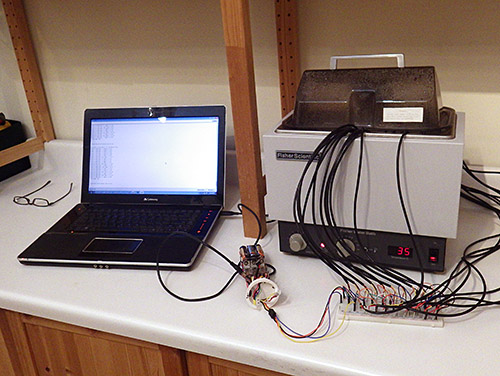
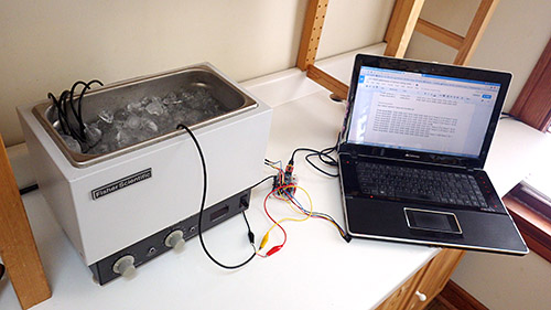
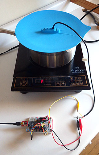
To see exactly how much of a factor this was for my loggers I mounted the LM303 sensor board in one of the underwater housings (which had a 6xAA battery pack about 10 cm from the sensor) and ran another test. The results made it pretty clear that, yes, magnetometers really do need to be calibrated inside their final operating environment. This also showed me that unless I was willing to spring for expensive degaussed batteries, I was going to need software that could provide significant soft iron compensation: the max & min only approaches just weren’t going to cut it. And I need to make sure that the battery & sensor orientations don’t not change during deployment by adding an internal brace to keep things from shifting around. It also occurred to me that there might be some temperature dependencies, but by this point I didn’t want to look under that rock and find there was even more work to do.

The top handle swivels, while the bottom is fixed

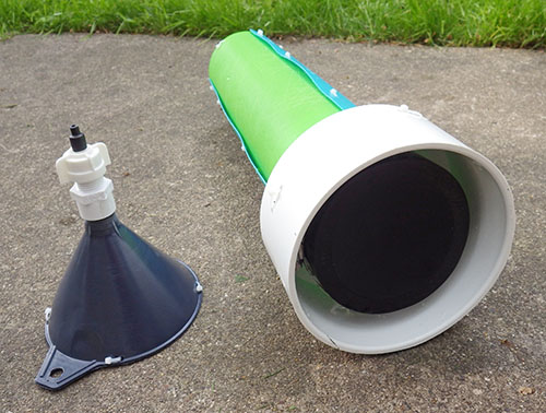
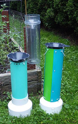
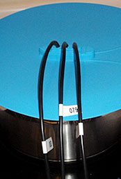
After seeing that plot I went back to the idea of building a geodesic frame big enough to contain the whole flow sensor, that could be assembled with zip-ties for transport into the field. And I think I found a way to build one out of tubing, but in the end I simply fashioned a couple of handles that could be connected directly to the threaded ends of my underwater housing. A sliding joint on the top handle allowed me to spin the unit slowly and smoothly as I pivot my body into different positions. The whole process takes about 10 – 15 minutes, using my arms as the calibration jig. This produces a spread of points that look like the blue line plot below:

Plotly again, with lines rather than points to show the pattern in the data as I twirled the unit about its long axis with the handles. This method only spins the unit around the Z axis, which shows quite clearly in the data.

Plotly again, with lines rather than points to show the pattern in the data as I twirled the unit about its long axis. This method only rotates the unit around the Z axis, which shows up quite clearly in the data.

Although this is not the same pattern you get from a 3-axis gimbal rotation, I am reasonably confident that I have captured enough points for a decent calibration. And the handles are easily transported so that I can do some post deployment calibrations in the field on the various different housings.

Although I was still boggled by forum threads discussing the finer points of “Li’s ellipsoid algorithm”, I still had to choose some software to generate the correction factors and I wanted something flexible enough to use with any compass rather than a one-of solution that would leave me tied to a specific sensor.

The best Arduino script  example of compass calibration I could find was the Comp6DOF_n0m1 Library  by Noah Shibley & Michael Grant (and I will be cribbing heavily from their integer trig functions for roll, pitch & yaw…)

Using the FreeIMU GUI Toolset

A post in Adafruits support forum suggested Varasano’s FreeIMU Calibration Application.  The FreeIMU calibration app was written with a GUI, but fortunately Zymotico posted a Youtube video guide that shows how a couple of simple config file edits let you run the FreeIMU GUI Toolset in manual mode:
(These are screen shots from that video)

FreeIMU_VideoScreenCap1

FreeIMU_VideoScreenCap2These changes allow you to run the application without the GUI, so long as you provide a couple of tab delimited text files of data.  The video goes into some detail showing how to use a processing sketch to save serial output from Adafruit 10 DOF IMU as a csv file, but all I did the first few times was copy and paste data directly from the serial window into a spreadsheet, and from there into notepad. (since my units are data loggers, I could use the csv files on the SD cards for the in-housing tests I did afterwards)

FreeIMU_VideoScreenCap3 Then you save “acc.txt” and magn.txt” in the FreeIMU GUI folder, right beside the freeimu_manualCal.bat file that you modified earlier. Once you have your data files in place, run “Freeimu_manualCal.bat”. On my machine the GUI still launches – displaying no data, but a command line window also opens:

FreeIMU_VideoScreenCap5

Note that if you try to run the batch file that you modified with the default data files the program came with you will see NAN (not a number) errors.  This is a sign that you did not save your new data files in the right directory, or that your data does not have the correct format. Once you have the FreeIMU Offsets & Scale factors in hand, the calculation is simply:

CalibratedData = ( unCalibratedData – Offset ) / Scaling Factor

When I used this procedure on the battery distorted data from that first housing trial the before and after plots looked like this:

LM303 magnetometer data, showing Before and After results with freeIMU calibration factors.

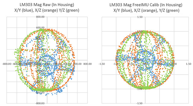
Now that’s what I wanted to see!  Even better: FreeIMU generated corrections for both the accelerometer and the magnetometer at the same time. (Units are lost when normalizing the ellipsoid because of the scaling factor. You can get acceleration back by multiplying by 9.80665 m/s*s.)

Unfortunately FreeIMU also comes with a whopping 300MB folder of support files, and with Fabio Varesano’s passing there is a real question about whether his software will continue to be available (or how long it will be updated to prevent some python version dependency problem from cropping up). I have also run across some scary looking hacked pages in the old varesano.net site, so it might be safer to use the wayback machine to search through it.

Using Magneto v1.2

My search for alternatives to FreeIMU lead me to Magneto v1.2 over at the Sailboat Instruments blog  That software was recommended by some heavy-hitters at the Sparkfun and the Arduino Playground forums, with one helpful person posting a step by step guide to Calibrating the LM303 with the Magneto software. With my earlier tests, I already had raw magnetometer data in text file, but I did not get good results until I noticed that before Scirus launched Magneto he was preprocessing the raw magnetometer readings with an axes-specific gain correction (See Table 75: Gain Setting on datasheet) to convert the raw output into nano Tesla:

Xm_nanoTesla = rawCompass.m.x*(100000.0/1100.0);
// Gain X [LSB/Gauss] for selected input field range (1.3 in these case)
Ym_nanoTesla = rawCompass.m.y*(100000.0/1100.0);
Zm_nanoTesla = rawCompass.m.z*(100000.0/980.0);

Save this converted data into the Mag_raw.txt file that you open with the Magneto program. Then your numbers match the magnetic field norm (or Total intensity) values that you get from the NOAA or BGS sites:

TotalField

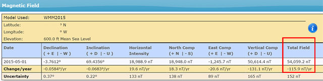
To use his method with a different magnetometer, you would have to dig into the datasheets, and replace the (100000.0/1100.0) scaling factors with values that convert your specific sensors output into nanoTesla. On the LM303, that factor is different on the Z axis than it is on the X & Y axes. But according to the author on the Sailboat Instruments site you only need to match the total field “norm” values if you want the final output on an absolute scale:

“Magneto expects to receive raw data in +- format (a value of zero indicating a null field in the current axis), but not necessarily normalized to +-1.0.

If your sensors have SPI or I2C outputs, they will usually directly produce the required format. For example, the MicroMag3 magnetometer directly produces counts from -3411 to +3411, and the the SCA3000 accelerometer directly produces counts from -1333 to 1333, and Magneto can process directly these values, without the need to normalize them to +- 1.0. I understand that a normalization may be desirable to avoid machine precision problems, but this has not been the case with these sensors.

If your sensors produce voltage levels that you have to convert to counts with an ADC, you have indeed to subtract a zero field value from the ADC output before using Magneto. You would then normally choose the maximum positive value as input to the ‘Norm of Magnetic or Gravitational field’.

But this norm value is not critical if all you want to calculate later on is a heading (if it is a magnetometer) or a tilt angle (if it is an accelerometer). You can input any reasonable value for the norm, the correction matrix will be different by just a scaling factor, but the calculated heading (or tilt angle) will be the same, as it depends only on the relative value of the field components. The bias values will be unchanged, as they do not depend on the norm.

Once I had my raw readings at the same scale as the Total Intensity numbers, I could hit the calibrate button, taking care to put the generated correction factors in the right section of the matrix calculation code:

Using Magneto1Rather than simply finding an offset and scale factor for each axis, Magneto creates twelve different calibration values that correct for a whole set of errors: bias, hard iron, scale factor, soft iron and misalignment. As you can see from the example above, this makes calculating the corrected data a bit more involved than with FreeIMU. I am not really sure I want to sandbag my loggers with all that floating point math (mistakes there have given me grief in the past) so I will probably offload these calculations to post processing with Excel.  To check that your calculations are working OK, keep in mind that in the absence of any strong local magnetic fields, the maximum readings should reflect the magnetic field of the earth which ranges between 20 and 60 micro-Teslas.

When I ran Magneto on the same data set I tested with FreeIMU, the x/y plots were once again transformed into perfect spheres, centered on the origin. Since I could not determine which software had done a better job by looking at the graphs, I took a hint from the Scirus post and decided to run the post-calibration numbers from each application as input to both programs. Since the FreeIMU “normalized” to unitless +-1 values, I had to multiply it’s output by my local 54,000 nT total field to use it’s post calibration output in Magneto. As you might expect, each program thought it’s own output file was perfect, requiring no further offsets, etc. But Magneto thought there were still “slight” offsets in the corrected data from FreeIMU, while FreeIMU thought the output from Magneto’s corrections were fine. I have slight in quotes there, because Magneto’s suggested bias corrections to the post FreeIMU data amounted to less than 0.1% of the total range. Given all the real world factors that affect compass readings, I’d say the two calibrations are functionally equivalent, although I suspect Magneto can deal with more complicated soft iron distortions.

What about the Accelerometers?

A side benefit of all this is that both programs can be used to calibrate accelerometers as well!  FreeIMU does this right from the start, producing unit-less +-1 results. For Magneto you might again need to pre-process your specific raw accelerometer output, taking into account the bit depth and G sensitivity, to convert the data into milliGalileo. Then enter a value of 1000 milliGalileo as the “norm” for the gravitational field. (Note: With the LM303 at the 2G default settings, the sensitivity is 1mg/LSB, so no pre-processing is needed. However the 16-bit acceleration data registers actually contain a left-aligned 12-bit number with extra zeros added to the right hand side as spacers, so values should be shifted right by 4 bits – which shows up as dividing by 16 in the Scirus example)

Now that I finally have a way to calibrate my sensors, I can move on to calculating the vectors for my flow meters. Being able to derive the sensors an instantaneous yaw angle from the magnetometer data would means that I no longer need to worry about the physical orientation of the sensors to calculate windrose plots  with circular averages. Of course bearing calculation brings me right back into the thick of the Quaternion vs Euler Angle debate, and I have more homework to do before I come to grips with any of that. But I also have so much soldering to do…perhaps I’ll deal with it “later” 🙂

Addendum 2017-04-20:

A pingback put me onto a long discussion at Pololu of someone working their way through tilt compensation on an LM303. They mention the use of MagCal, another software option which confusingly, outputs the INVERSE of the matrix that you get from Magneto. But there are tools to flip the matrix if that is the software you have available.

Addendum 2017-10-12:

Accelerometers are so jittery, that it’s always a good idea to read them a few times and average the results.  Paul Badger’s DigitalSmooth does an excellent job when you feed it 7-9 readings for each axis. This filter inputs into a rolling array, replacing the oldest data with the latest reading. The array is then sorted from low to high. Then the highest and lowest %15 of samples are thrown out. The remaining data is averaged and the result is returned, allowing you to calculate things like tilt angle.

Addendum 2018-04-11:

Posting a quote here from jremington, as several people have emailed questions about IMU’s, which add a gyro into the mix.

“The accelerometer is used to define pitch and roll (while the craft is not accelerating or rotating), while yaw is defined by the magnetometer. Another way to look at this is that the magnetometer defines the North direction, while the accelerometer defines the Down direction. North and Down are combined to generate East, for a full 3D coordinate system called North East Down (NED). Both of these sensors are required to determine absolute orientation. The gyro only measures rotation rates and cannot be used to define any angles. It simply helps to correct for the fact that the acceleration vector is not g (Down) if the craft is rotating or accelerating.”

Again the place to start reading about IMU’s is probably the CHrobotics library. And I’ve heard rumors that the MPU6050 with the i2cdevlib DMP example sketch generates both quaternions and sensor-fused motion data at ~100Hz, so that might be a good code reference…

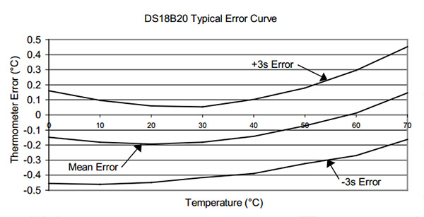
Addendum 2023-12-01: A quick testing platform for your sensors

People are not likely to jump into building underwater units immediately, so you’ll need a platform to test the different accelerometers on the market. Our 2-Module Classroom data logger is probably the fastest way to get a testing fleet together, with mini breadboards making the sensor swaps effortless. Even relative power hogs like the ADXL345 should be OK for a few weeks of operation with the 1000µF rail buffer.

Field Report: 2015-03-23 Flow Sensor “drag fins” tested

Our deployments last year saw only modest instrument response in slower systems, especially those where the water was flowing slower than 1 cm/second. Most of the deep saline circulation fell into this category, and we really wanted better data from those caves. So I came up with a add-on attachement for the flow meters, hoping to dramatically increase their surface area without affecting buoyancy that much.

Officially this was an introduction to beach facies mapping, but it looks more like geosci Kung Fu to me.

Technically, this was an introduction to mapping beach deposits, but to me it looked like geo-scientist Kung-Fu

I had a couple of these new fins on this trip and I asked my wife, who was busy leading the Northwestern University earth science students around the peninsula, when I might sneak away from the group for a few hours to see if they actually worked. She suggested instead that we do an actual deployment, using the opportunity to expose the undergrads to the aspects of real underwater fieldwork.  I was instinctively cautious about this idea, having seen a fair number of tech demos go wrong over the years, but I have also come to realize that Trish’s enthusiasm is an unstoppable force, so we added the dive to a schedule that was already bursting.

The new "parallel" anchor rig make the differences between the instruments obvious...

The new “parallel” anchor rig made it easy to see differences in instrument response from the last deployment. It’s hard to achieve consistent results with all the changes I make from one generation of underwater housings to the next.

With all the other activities on the go, it was mid- afternoon before we actually donned our gear, while answering questions from the students about the double tanks, and doing little demos of the other cave-diving kit. Then we waddled off to the waters edge, festooned with the mesh bags of loggers, cables, and other bits that accompany a typical deployment. I’m not saying we looked bad, but it was probably clear to the students that we weren’t going to peal off and reveal a freshly pressed tuxedo after the dive 😉  Once in the water, we had a short swim along an open channel to the cave entrance with a gaggle of snorkeling students following our progress at the surface. One of our primary lights started acting a bit flaky on the way and we had another impromptu Q&A session floating among the mangroves as one student paddled back to fetch our spare.  A bother, but it did put a point on what we had said earlier about all the redundant equipment we were carrying. When the extra light arrived, we started the dive, and I made a note to myself to take more photos than usual for the debrief that would occur at the end of the day.

Here I am adjusting the ballast on one of the flow meters before deploying it.

Here I adjust the ballast mass on one of the flow meters before installation (with the new drag fin in the foreground)

Once on site, Trish set our mesh bags up in a little work area, and I swam out for the usual round of inspections. North? check. Epoxy OK? check. Vortex shedding? etc. Once that was in the dive notes, I began the one-by-one exchange of the old units.  The indicator LED’s pipped right on schedule, telling us that we had no epoxy failures this time round. Once all the flow sensors had been replaced, I took a few photos and noted that the unit closest to the main line was not being deflected as much as the other sensors. I then added the new drag fin to that heavier unit.  I also had a pressure sensor to install, and while I switched that out I could see that the sensor with the new drag fin was now almost horizontal compared to the other sensors:

I don’t know about you, but I am calling that a success.  In faster systems the fin might clip the high end, although the cross sectional area now changes quite a bit as the unit approaches 90 degrees. Any approximation with drag on a sphere has also gone out the window, but I already knew that empirical testing was going to be necessary to get point velocities. As I refine this idea, I will come up with different sizes, and integrate the baffles more elegantly with the ballast mass adjustment. Wheels are already turning in my head with possibilities.

Addendum:

As part of the extra video we captured for the students, I recorded a short clip of our exit from the cave. With the water at high flow, there was significant mixing at the fresh/salt water interface, producing an optical consistency similar to salad dressing. This is limited to the mixing zone region, and you can see this when I placed the camera below the level of the interface where it obtains clear visibility again.  While cave divers run into this kind of thing frequently, it’s probably something that regular divers don’t experience very often. So I thought I would post the clip just to show people what it was like:

<— Click here to continue reading the story—>

Field Report: 2015-03-18 One logger sacrificed to the sea gods.

DIY Cave Pearl data loggers based on Arduino Microcontrollers

The B4 unit has been a star performer despite the fact that it was one of the earliest logger units I ever built. It has been running continuously since its first cave deployment in March 2014.

I was happy to see Gabriel from CEA the next morning to discuss retrieval of the open water units, but he delivered some unwelcome news to go with my morning coffee: the logger at the mouth of Yalku Lagoon had gone missing. Loosing the unit itself was irritating, but loosing four months worth of data – that hurts!  Another pivot joint on one of the loggers in the bay had failed the week before, and one of the reef volunteers spotted that unit while it was still hanging from the backup bungee. I received that news before we headed south so I had quickly crafted some stronger universal joints from pvc to fix the problem. It was salt in the wound to know that these new pivots were sitting in my suitcase, having arrived a day or so too late to save the Yalku unit. Darn!

Oh well, we can only try again, and there is some solace in the fact that we are not the only ones to see equipment suffering this fate.  There is still a small chance that someone will pick it up further down the beach, try to figure out what it is on Google, and send us an email to say they still have the SD card. From this point forward, I will be labeling the inside of my loggers as well as the outside, and I will add a little “If found please email…” blurb into the data files.

Marco cuts B3 from it's mooring

Marco cuts B3 from it’s mooring on the south side of the bay. Marco has been doing regular checks on the loggers since the beginning of the open water experiment.

Gabriel had meetings to attend, so Everett, Marco and I popped on some fins and swam out to recover the units in Akumal bay.  As usual they were covered with a crop of algae & other critters but both B4, and the B3 unit that I rebuilt on the last trip, were still running smoothly. The unit in shallow water was so encrusted that I told Marco to pull the whole assembly, including the anchor plate, because there was no way to inspect it through all the accumulated cruft. That bio-fouling likely increases the drag and the buoyancy of the meter over time.


I left one of the new pivot joints on the B4 anchor plate. Hopefully these are robust enough for the constant wear and tear.

This is one of the new universal joints – hopefully robust enough to save us from more losses.

These two loggers have now been in the open ocean for seven months, and once ashore I began a familiar routine, cleaning them with green scrubby pads and copious amounts of rubbing alcohol.  The Loctite E-30CL epoxy on the LED’s is holding up well although the JB weld on one of the DS18b20 temperature sensors definitely has little patches of rust showing through. The stainless steel ballast washers appear to have fused together, but the O-rings are still looking good. The nylon bolts are sounding crunchy, perhaps indicating that they are starting to get brittle so I might replace them on the next round.  Now that the new pivot joints are more robust, I probably need to think about upgrading the rest of the connections as well.


JB weld on one of the DS18b20 sensors

The JB weld on the DS18b20 sensors is getting a bit crusty.

Once the data was downloaded, I reset the RTC’s, and checked that the sleep currents were still the same as they were in December. These units have Tinyduino stacks, so they run with fairly high sleep currents. (around 0.7 mA) With six new AA’s in the power module they should still deliver 6-9 months of operation.  After adding a fresh desiccant pack they were sealed & ready to deploy with code that crops the highest and lowest off of 13 readings, spaced 8 seconds apart. I average the remaining 11 readings to filter out the high frequency wave turbulence, and get at the underlying flow direction. So far this approach seems to be working well.  I also gave Gabriel a new logger to replace the one we had lost at Yalku lagoon Hopefully the sea gods will smile upon this new deployment.

<— Click here to continue reading the story—>

Field Report: 2015-03-17 Drip Logger Service Visit

Everett was one of the grad students who also came down to help with the N.U. trip.

I pressed Everett (a Northwestern grad student) into helping me with the manual counts when I collected the drip loggers.

In March my wife led a Northwestern University earth sciences trip to the Yucatan Peninsula. While she was busy with all the necessary preparations for the students who would be arriving shortly, I slipped away for a couple of hours to retrieve the loggers we left at Rio Secreto last year. With so many new units in that deployment, I was really chomping at the bit to see how they faired.

As usual we had some good news, and some bad news from the deployed loggers. Actually, we probably set a new record on the bad news side of things as the two relative humidity loggers that I cobbled together before the December trip went bananas as soon as we brought them into the caves. The HTU21D sensor on unit 030 died on Dec. 20th, one single day after it was deployed, while the sensor on 028 lasted for four days before it pooped out.  Both delivered crazy readings the whole time even though they seemed to be working fine on the surface.

capt

Even potted under epoxy, the solder contacts were severely oxidized.  I suspect that moisture was able to “creep” along the surface of the breakout board, because of the area exposed around the humidity sensor.

The epoxy in the sensor wells had turned yellow & rubbery, even though it was clear and rock hard when the units were deployed . But these sensor caps were assembled just days before the flight, and I used 5 minute epoxy to speed the build, rather than the usual 30 minute stuff. So I am thinking that the moisture resistance of the faster curing epoxies is much lower. Perhaps it’s time for me to investigate some new urethane options with lower permeability? It is also possible that PVC solvent residue interfered with the epoxy’s chemistry because I built them so quickly.


Dispite its "splash proof" rating, this MS5805-02 quit after one month in the cave

Despite its “splash proof” rating, this MS5805-02 died after one month  in the cave. It had no “direct” water contact.

The loggers kept running after the R.H sensors stopped working but they eventually both quit long before draining the AA battery packs, which leads me to conclude that rusty contacts eventually shorted the I2C bus, preventing the RTC alarms from being set. We also lost one of the pressure sensors, and a TMP102 board. In fact the only sensor still fully operational when I pulled the loggers was the MS5803-02 pressure sensor, once again showing just how robust those pressure sensors are under their white rubber caps.


PressureSensorOnPalaparoof

The white ball is an older first gen housing for an underwater pressure unit, and the black cylinder above is a drip sensor, acting as a crude rain gauge. I don’t know who collected the rain water.

I left a new RH&Pressure unit in the cave, which was made with E30CL and had more than a month of test runs under its belt before going into the field. Even with fully cured epoxy, there is still the possibility that moisture will penetrate through the exposed RH sensor, so I will look into moving that sensor off the main housing for my next builds.

We also had some sensors on the surface during this last deployment, and they faced dramatically different challenges under the full tropical sun.  The pressure logger had been re-purposed from a four month cave deployment. It sported a DS18b20 temp sensor, and an MS5803-05 pressure sensor, which both performed beautifully in the underwater environment.

But as you can see from the pressure record (in mBar) things did not go so well this time around:

DIY Cave Pearl data loggers based on Arduino Microcontrollers

I was expecting daily fluctuations of a few millibars so there is no way I can believe that local highs reached 1200 mBar…but what happened?  This pressure sensor had been used first for an under water deployment so it had a layer of Qsil silicone over top if it. This caused a -50 mbar offset, but did not seem to give us any other problems in the thermally stable cave environment.  But with full sun exposure this logger saw huge daily temperature variations (detailed below) I believe this caused the silicone above the sensor to expand and contract; exerting enough physical pressure to overwhelm the more subtle barometric readings. Unfortunately I did not have time to look at this data while we were in the field, so the unit was redeployed, although this time in a more sheltered spot under the palapa roof.

Now for the good news:

The drip sensor which we left beside that pressure logger on the surface delivered a respectable record despite the fact that it had no collecting funnel:

DIY Cave Pearl data loggers based on Arduino Microcontrollers

That peak of 8000 counts (/15 min.) is about 9 drips per second on the surface of the unit which, with all the delays I put in the code to suppress double count artifacts, might be approaching the max response of the sensor itself. With no way to capture the water, gentle foggy rain events would not have triggered the impact sensor, so there is a good chance that a significant amount of precipitation did not get recorded. But what makes this record so impressive to me is the RTC temperature log from inside the housing:  (in °C)

DIY Cave Pearl data loggers based on Arduino Microcontrollers

The black end cap actually started melting grooves into the white PVC of the drip logger housing.

The black end cap actually started melting grooves into the white PVC of the drip logger housing.

The spec sheet maximum for the DS3231 is 70°C,  and the Arduino mcu‘s limit is 85°C.  Even so, with daily peaks reaching nearly 60° I am quite surprised that the batteries did not pop.  The little logger did not escape this trial by fire completely unharmed, as the micro SD card went from a nice low current sleeper to pulling around 1 mA all the time. The data was intact, but I can only surmise that the high temps cooked some of its control circuitry. The upper ABS surface also changed from a neutral frosted white to a slightly fluorescent green/yellow color, presumably because of intense UV exposure. After replacing the batteries & SD card, the unit was put back on roof for another run.  Just to be on the safe side I added a second unit in case that first one gives out.

While I leave heavy weight analysis of the hydrographs to the expert on the team, I couldn’t help peaking to see if these surface storms affected the in-cave drip flow rates. I was quite surprised to see that the precipitation events had small effects on some of the counts, while barely registering as a blip on others that were quite nearby. This is the record from DS20 (15 min bins, with a purple overlay of surface record that is not on the same scale):

DIY Cave Pearl data loggers based on Arduino Microcontrollers

And this is the record from DS02, located less than 5m away in the same chamber:

DIY Cave Pearl data loggers based on Arduino Microcontrollers

Given the thin soils of the area,I suspect that much of that brief rain evaporated shortly after surface contact, or the dry season vegetation was just sitting there like a sponge, able to absorb most of it quickly.

The whole group of loggers represents a mixed bag of first and second generation builds with many different “mini” form factor Arduino boards in them. I left the batteries in a couple of units back in December so I could see some longer term battery discharge curves:

DS01_02_Longruntest

These two units were using three lithium AA’s, which I knew from the 1st generation test results, are about 2/3 depleted when they hit that 5000 mV shoulder. This tells me that DS01 would probably have delivered nine months of operation on these cells. This is very good news because even the loggers I built with no-name eBay clones (MIC5205 v.regs) sleep around 0.33 mA if they have good SD cards. So it should be safe to put them on a six month rotation schedule.

In addition to their drip counts, several of the loggers were running with different eeprom buffering levels to help me understand how this affected the power budget. I won’t wade into all of that data here but two of the most directly comparable records are from units 26 &  27:

Logger # starting voltage sleep current
# records buffered  V.drop/8500 records
26 5243 mV 0.28 mA 512 30 mV
27 5198 mV 0.26 mA 96 33 mV

Unit 26 was handicapped by a slightly higher sleep current and a starting voltage above the lithium plateau (I often see a small quick drop on 3xAA lithiums above 5200 mV) The fact that it still delivered a smaller voltage drop on the batteries over the three month run implies that increasing the size of the eeprom buffer does improve performance. Logger 26 had a 32K eeprom so it only experienced 16 SD card writing events, while the smaller 4K buffer on unit 27 required 87 SD writes.  Both loggers created six separate log files during the run and the cumulative drip counts were comparable.  It’s still a close call, and the increased buffering does not providing a huge savings, perhaps on the order of 5-10%.  Since the extra I2C eeproms only cost $1.50, and the coding to support them is trivial, I consider that to be an easy way to get another month of run time. As with the buffering tests I did back in 2014, it’s clear that all those eeprom page-writes (3mA x 5msec  + mcu uptime) take a significant amount of power. But at least they are not subject to the random latency delays you see with SD cards.

I added larger LED limit resistors to each logger on this service visit, so even if the drip rates pick up dramatically during the wet season, power used by the interrupt will be reduced compared to the runs since August. All units that were capable are now buffering about five days worth of data to the eeproms. The current crop of “best builds” with Rocket scream boards and pin-powered RTC’s, are getting down to 0.15 mA, implying that they should be good for a year long deployment provided the SD cards & sensors hold out. Of course I don’t count chickens anymore, no matter how good the numbers look. Though all units delivered a full data set on this deployment, two of them suffered dramatic increases in sleep current when their ADXL’s suddenly started consuming more power. You can easily spot when these kind of sensor failures occur by looking at the power supply voltage log:

020_SleepCurrentChange2

I am sure there are more gems buried in the data, which I will post here as they are uncovered.

<— Click here to continue reading the story—>

Calibrating DS18B20 1-Wire Sensors with Ice & Steam point measurement

You will need to crimp the ends and give each sensor a serial number, but don't label the sensor itself as I have in this photo or the will fall off during the steam point testing.

Give each sensor a serial number, but don’t label the sensor itself as I have in this photo or the labels will just fall off during the steam point testing. After adding crimp pins to the wire ends it becomes easy to gang them together on a breadboard for testing. Despite Maxim’s warnings, I had star configurations above 20 sensors reading well with them close together like this.

I’m probably not the first person to note that sensor calibration is one of the big differences between the mountains of data coming from the citizen science movement and that produced by research professionals. (…mea culpa…) After opening this can of worms, I think I am beginning to understand why: Accuracy calibration rapidly gets complicated, or expensive, and often it’s both at the same time. By the time you have what you need to do the job, the difference between a $0.30 sensor, and a $30 sensor, is pretty insignificant. So it’s no surprise that few people work on calibration methods for low cost sensors, or why normalization approaches are used instead.

But I am already spending far too much on this little hobby, so despite knowing that the folks over at Leighton Telescope managed to get their DS18b20’s to about ±0.01°C with a NIST traceable thermometer, I thought I would see how far I could get on my own.  I suppose if I was an alpha geek,  I would make my own platinum RTD  and calibrate the sensors against that.  But I’m not quite there yet. I should also point out that numbers are not my strong suit, so there could be some significant errors in what I have cobbled together here and I appreciate any feedback to help correct those…

The first thing that occurs to me is: Can you read the temperature more accurately  by averaging a bunch of these sensors together?  If the readings from the sensors have a mean and standard deviation, then as the number of sensors increases then the standard deviation should decrease…right?  The data sheet gives you a sense of how far you can get with that approach, because I assume that Maxim/Dallas used a very large number of sensors to derive their typical performance curve:

DS18B20_TypicalPerformanceCurve

But if I understand what people say about this graph, the only reason the 3 sigma spread on that graph looks better than ±0.5 at 20°C is because the errors in the sensors used to derive that curve were truly random, and had a nice Gaussian distribution around that mean. However, since the actual batch of sensors I am holding in my hand is likely from the same production run, it is subject to systematic errors that don’t cancel each other out so nicely. And since I bought them on eBay, there is also a chance that they might be fake DS18b20’s.  So I could have no idea how my mean error line was related to the one on Maxim’s graph.

But there are still useful things you can do with this kind of averaging:

test

The front temperature display on this clunky old Fischer Scientific was off by more than 2°C, and it was missing a foot. While it’s hardly a temperature chamber,  the insulation and covering lid produced a slow cooling curve, so I could be reasonably confident the sensors were being exposed to the same temperatures. Don’t use data from the rapid heating cycle, because temperatures are likely to be unevenly distributed in the bath.

First of all you can get rid of the bad sensors by selecting a group that has a consistent behavior over the temperature range you are looking at, with readings that fall within the manufacturer’s specifications.  To get enough data for this kind of assessment, I needed to run at least 10 sensors at the same time so that the average had some statistical weight. For this testing I picked up an old five Litre isotemp bath (you can find them for $25-$50 on eBay) but you could just as easily do this with hot water in a styrofoam cooler. With about 20 sensors on a breadboard in a star configuration (4.7k pullup), I brought the water bath up to a stable 40°C, and then moved the entire thing out into the fridge and left it logging during the cool down. The lid was on, and I had several towels over top to make the process go as slowly as possible.  It took 12 to 24 hours for each batch of sensors to reach ~5°C.

With this data in hand, I looked at the residuals by subtracting each sensors raw reading from the average of all the sensor readings.  This exercise sent one DS18 straight into the bin, as it was more than 2.5°C away from the rest of the herd for its entire record.  Another was triaged due to a strange “hockey stick” bend in it’s residual around 25°C.  I threw out the data from those two duds, and recalculated the average & residuals again.  Just to be on the safe side I decided not to epoxy any sensors into a long chain if they were more than 0.3°C away from the average. (although I am still wondering whether eyeballing residuals like this is enough to exclude the right outliers?)

You can then normalize the sensors to each other by fitting a quadratic equation to a graph of each sensor & the overall average line. Excel can generate these coefficients for you with the linest function, or it can solve the quadratic with Goal Seek.  But the easiest method I found was make a 2nd order (but not higher) fit with the chart tool’s trendline function. Make a scatter plot of the data with the averages on the Y axis, and data from one individual sensor on the X axis.  Then right click on the data points to select them, and choose ( Add Trendline ) from the pull down menu, with the [ ] Display equation on chart tick box checked.      (here is an example of the technique using an older version of Excel)

The equation you see displayed will convert that particular sensors output into corresponding temperatures on the average line. With this transformation, each sensor will yield the same reading if it is in the same thermal environment, and you can accept that any differences between two sensors in the chain represent real differences in temperature.

This kind of normalization is as far as most people go. However for the reasons I outlined above, we can’t be sure that we were using a valid sample for that mean data. In my tests it looked like I did not have an equal distribution of sensors above and below the average line, so I still didn’t really have a handle on whether this was improving the absolute accuracy. (I will post some example graphs of this later…)

That brought me to calibrating the DS18b20’s against intrinsic physical standards which rely on the fact that during a phase change  (melting, freezing or boiling)  adding and removing heat causes no change in temperatureIn fact those heating curve plateaus are known so precisely that they use them at NIST to calibrate the expensive thermometers that I am trying to avoid buying.  Today they do this with Gallium‘s triple point (29.7666 °C) and the triple point of water (0.010 °C), but they used to use Gallium’s melting point plateau. (29.7646 °C)  Gallium sells for less than a buck a gram on Amazon and a density of about five grams per cubic centimeter means a block big enough to surround one of the DS18’s is almost within a DIY’ers budget. (100 grams will make a disk about two inches across and a quarter inch thick) But considering that commercial Ga melt cells cost about three grand, either that stuff is nasty enough to get me into trouble, or you need allot more more of it, at higher purities than you can buy on eBay to build one.  Then there is the significant time it would take to refreeze the block again for every single sensor. And finally, all exposed metal must be carefully lacquered as Gallium will form an amalgam with many metals, and any dissolved metals will compromise the purity of the bath, shifting the melting point. And you would probably have to cover everything with Argon wine preserver.

So I went hunting for other substances I could use for a mid range calibration point and found several good boiling points such as: Ether (35 °C), Pentane (36.1°C), Acetone (56 °C), and Methanol (66 °C). Despite my enthusiasm over coffee the next morning,  all of them were summarily rejected by my wife, who strongly suggested that I look for calibration procedures that do not create large amounts of highly explosive vapor. Given how unstoppable she usually is in the pursuit of  good data, I was not expecting this outburst of common sense 🙂

So I looked at the other primary standard used to calibrate pt100’s. Turns out it is possible to make your own triple point cell, and if that’s not good enough for you,  Mr. Schmermund also produced plans for a freezing point of mercury cell (–34.8 °C) (See: “Calibrating with Cold”, Shawn Carlson, Scientific American, Dec. 2000 issue).  However the local 7-11 was fresh out of liquid nitrogen when I checked, and I had this gut feeling that risking mercury induced brain damage was not going to pass the cost/benefit analysis either. If I actually did need sub zero calibration I think I would try using Galinstan, (−19 °C) which is now replacing mercury in glass thermometers.

If you can pre-chll the sensors in one corner of the bath, the whole process goes much faster.

Pre-chilling the sensors in one corner of the bath makes the process much faster. Hold the sensors by the cable, not the metal sheath, or heat from your hands will affect the readings.

It was looking like calibrating against anything other than distilled water was going to take a substantial amount of effort compared to what I was seeing in the NIST and EPA videos. Most sources indicated that the ice point and steam points were at least an order of magnitude more accurate than my ±0.1°C target, making them suitable for the exercise.

While the overall procedure is pretty easy, it did help to practice a few times to get a sense of when I could trust the readings. Checking that you have just the right amount of water in your ice bath makes a big difference, and don’t run the sensors at full tilt or they will self heat. (I left 15 seconds between readings) Since errors on my part would cause the sensor to be warmer than the true ice point, I took the lowest reading, while stirring, as my final reading. The difference between stirring, and not stirring was usually 1-2 integer points on the sensors raw output (0.0625-0.13 C) and this was consistent for all the sensors.

If these sensors were linear then reading the ice point was a direct measure of the b in y=mx+b. And this got me wondering if one point calibration was enough all by itself.  But once again my wet blanket science adviser assured me that nothing on those graphs told me if the offset was constant over the sensors range. Hrmph! (Although according to Thermoworks, ice point alone can be a good way to check for drift, because the most common error in electronic temperature sensors is a shift in the base electrical value)

I found a silicone vegetable steamer lid for the calibration that had three DS18B20 sized holes in it already.

I found a silicone vegetable steamer lid for the calibration that had three DS18B20 sized holes in it already.  Getting the right pace for your slow rolling boil is important, and this lid sheds the condensed water back into the pot reasonably well. Alligator clips also help speed the process.

So I moved on to measuring the steam point. Water’s boiling point is not necessarily at 100°C and the only factor that is really involved in the variance is atmospheric pressure. Altitude is often given as an alternative when pressure information is not directly available and there are plenty of places to look up elevation and barometric pressure data (& converters) for the necessary corrections.

I already had some MS5805-02 sensors on hand, so with the help of Luke Millers library, I could read my local atmospheric pressure for the correction directly.  The accuracy of my pressure sensor was ±2.5 mbar (similar to  the more common BMP180) with the B.Pt adjustment equation being: Corrected B.Pt.=100 (°C)+((PressureReading-1013.25mbar)/30)  So the 5 mbar total error range in the pressure sensor could change the adjusted boiling point by up to 0.166°C.  This means that the error in my pressure sensor measurement is at least as significant as the other aspects of this procedure. Better than the default ±0.5°C, but it puts a limit on how accurate I will can get with my steam point measurement.

Doing multiple sensors at once saves significant time, but be carefull or you will pay the piper with a couple of burn fingers

Cutting down the stacks on the Fred steamer lid allowed me to do multiple sensors at once. This saves time, but be careful or you will pay the piper with a few burned fingers when you change them out.

With each sensor just under the surface of the boiling water (since the evaporation process happens a little bit above 100°C) each one took about 5 minutes to warm up to reading temperature with the water on a slow to medium boil (and it was easy to see that on the serial monitor) I didn’t consider the test done till I saw at least a full minute of stable output (reading the sensor every 10 seconds) Since errors in my technique would produce readings on the cold side, I took the highest ‘frequently repeated’  number as the final reading. Most sensors settled nicely while some of them toggled back and forth by one integer point from one reading to the next.

In comparison to the steam point procedure, I trust the Ice point as more reproducible because it does not suffer from any pressure information dependency. Perhaps more important is the fact that 100°C is far away from my 20-30°C target range, leaving the possibility for significant errors if the sensors have a non-linearity problem.

With the ice and steam readings in hand, I could construct a two-point calibration for each of my DS18B20’s with slope M=Δy/Δx, and B=(the ice point reading).  (explained here, and that left you in the dust there are lots of fill-in-the-blank spreadsheet templates on the web)

At this point I am still doing tests & chewing on numbers, but the standard deviations around the mean line are being reduced by this ice&steam point calibration. The problem is that even after I apply the resulting slope and intercept I still have significant residuals from a mean that is derived with the corrected numbers. I thought that the two point calibration would make the graphs the individual sensors line up very closely with one another, and that they would have nearly identical slopes(?) I am left wondering if larger sensor errors up at 100°C mean that I need to apply some additional process to normalize my sensors to each other in the 30°C range after doing the two point calibration.  But using the process I described above would generate ‘b’ value corrections, and I am very reluctant to modify my y intercept numbers because I think using the ice point to measure that offset is robust. These doubts about accuracy of the steam point, the sensors linearity, and my lack of a nice “mid-range” standard to calibrate against, have me hunting for a method which would gracefully combine a single (ice) point calibration with normalization. And the dip in the datasheet’s mean error curve between 20-30°C implies that even after applying ice point corrections my average line will still be 0.05°C lower than actual (?)

Another important observation is that the means generated from the uncorrected data were within 0.14-0.16°C of the means calculated after applying the two point calibration. Either my sensors actually did have a reasonably normal distribution of error, or I might have missed something important.  The implication in that first case is that normalization alone should improve your overall accuracy, but I still need to get my hands on a calibrated pt100 to know for sure….Argh!

Addendum 2015-05-18

Bil Earl just posted a beautifully written article on sensor calibration, which puts everything here into context. A great job once again by the folks over at Adafruit!

Addendum 2016-02-12

Just adding a quick link to a small post on the pre-filtering I do with these sensors, which I only posted because no one else seems to bother posting data on the ‘typical quality’ you see with the cheep eBay sensors. And after splashing out on a Thermapen reference thermometer ($200), I can try a multi-point calibration for these sensors that is closer to my target temperature range.

Addendum 2016-03-05

Just put the finishing touches on a new calibration approach which, compared to this ice & steam point method, was an order of magnitude faster to do. If you are calibrating a large number of sensors, the reference thermometer is definitely worth the investment.