In this post we will describe a process of adjusting raw data from multiple temperature sensors to remove offsets for accurate comparison when they are deployed as a set. This is not the same as calibration which often uses references with exact physical values to improve accuracy. However, normalization is a highly complementary way to improve precision which can be vital when you are studying systems that are driven primarily by gradients. Sous-vide cookers are portable so this procedure can be done in the field with a mix of sensors from different vendors. Sensors that are not inherently waterproof can be sealed inside food vacuum bags during the procedure.
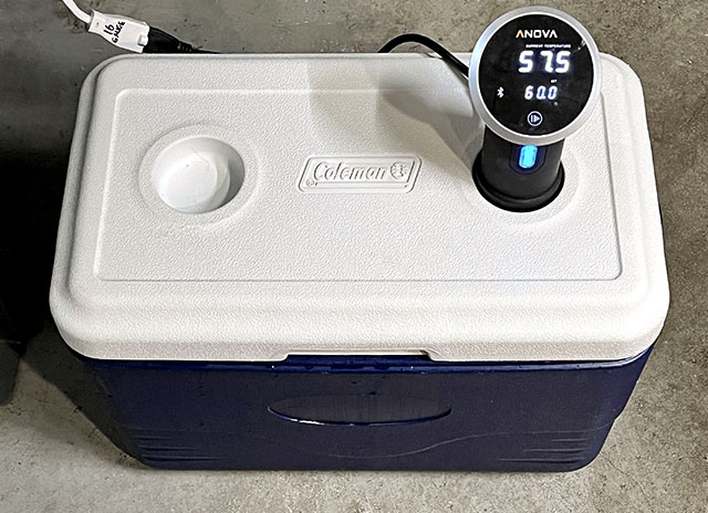
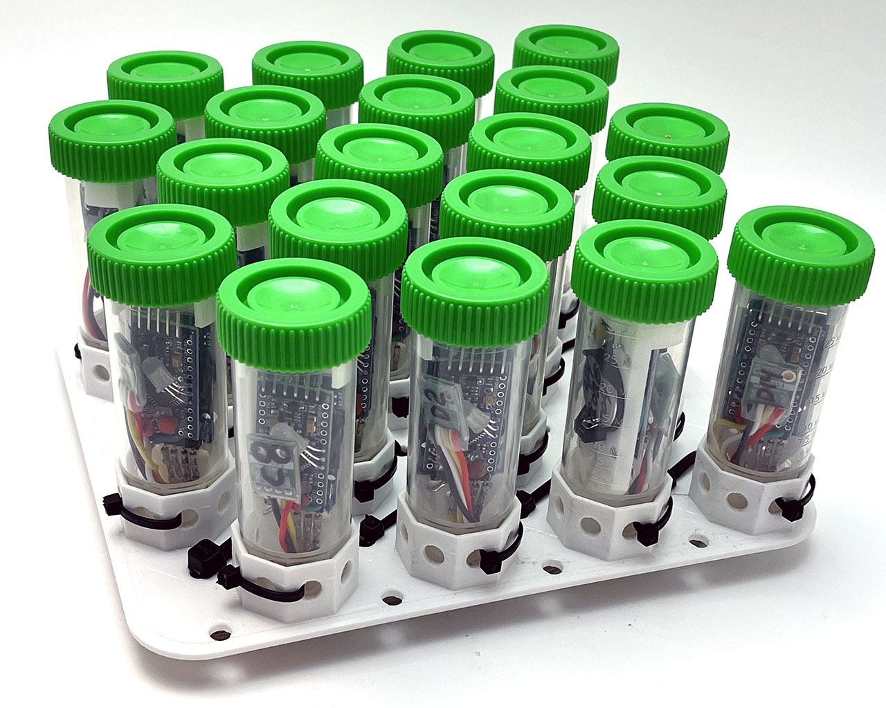
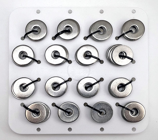
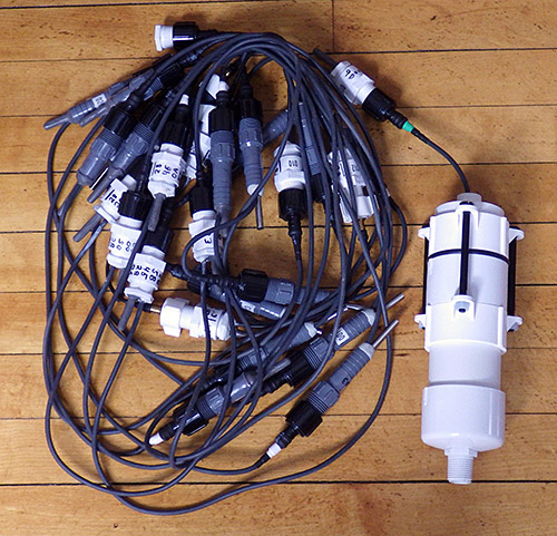
Here we used this rig to normalize as set of Si7051’s reference sensors that will later be for calibrating the NTC thermistors on every Cave Pearl logger. We have accumulated quite a few of those Si’s over the years and it will be interesting to see if the older ones have drifted. But this 48 quart cooler also has enough volume to enable normalization of the temperature sensors inside the larger PVC housings on our older generation of loggers.
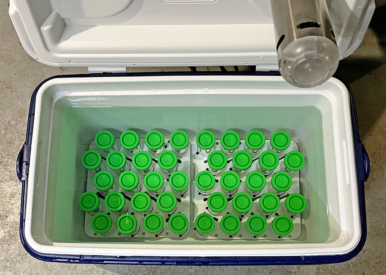
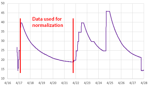
With the significant setup time, I created several ramps to provide some surplus data. Even with the thermal control of the Anova, I prefer to use the slow passive cooling curves whenever possible. With the circulator operating continuously the system took five days to cool from 40 to 20°C: slow enough to avoid any lag issues due to the housings or inconsistencies in the circulation.
Linear Y=Mx+B Normalization:
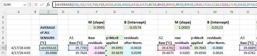
We have released many normalization tutorials over the years, but I will review the basic steps here for completeness. You start by drawing an average from your group of sensors. This will be the value each individual sensor gets adjusted to: (click to enlarge the images)
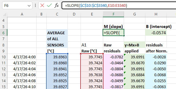
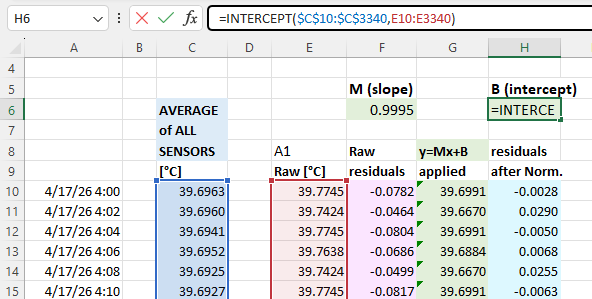
With that you calculate normalization constants using Excel’s slope & intercept functions with the columns of average & raw data for each sensor. Using these formulas lets you copy/paste the equations from one data set to the next which dramatically speeds up the process when you are working through many sensors. It also recalculates those constants if you add or delete information from the normalization set:
The next step is to calculate the difference (called residuals) between an individual sensors output and the average: you will do this both before and after the Y=Mx+B corrections have been applied to the temperature readings. These differences between the group average and a given sensor should be dramatically reduced by the adjustment:
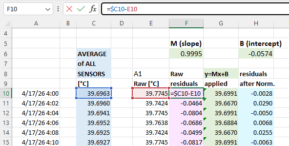
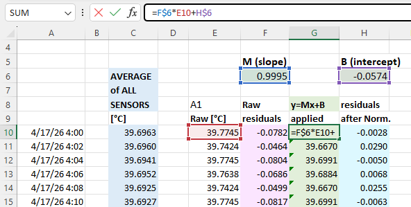
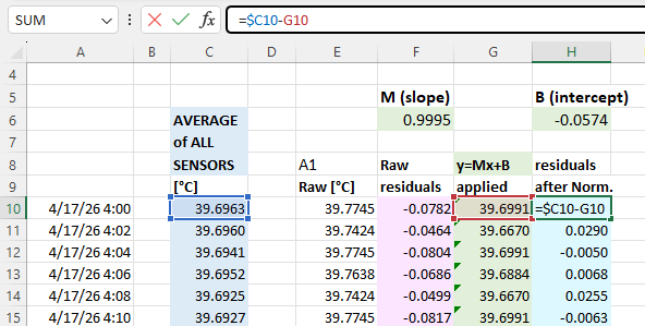
Then create scatter plots of the pre & post normalization residuals so you can compare them side-by-side. The adjusted residuals should have very little slope and be equally distributed around ZERO:
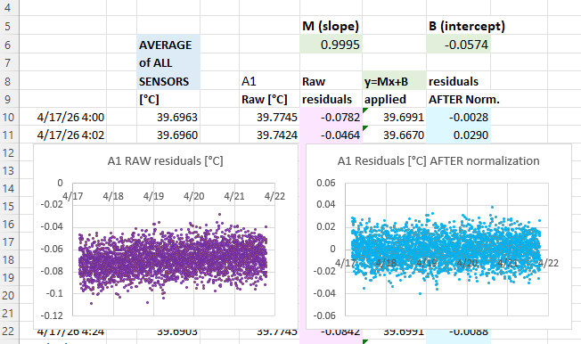
I should mention here how remarkable it was that this batch of sensors produced what I can only describe as textbook residuals with soft fuzzy distributions showing no observable patterns. Usually a batch of mixed sensors will show some structures in the residual plots – indicating that one (or more) of the sensors in the group has some kind of problem and might need to be removed from the group average. A failing sensor or connection issue should be your first suspect if you see step-changes in the residual plots when you know the physical system was changing slowly. If you can’t identify the misbehaving sensor to reject from a group, then you could normalize to the median rather than then average, as this tends to be more resilient to outliers.
A common source of problems during normalization is accidentally including data from a logger that has its timestamp offset from the rest of the group. This can be due to human error during setup but it also creeps in due to clock drift. In that case the overall pattern in the residuals plots will be a version of the same shapes you see in the raw sensor data. It’s often useful to have at least one deliberately induced ‘sharp’ temperature change in the raw data to align the raw data records.
Temporal alignment gets more complicated if your sensors have heavy physical housings causing excessive thermal lag compared to others a ‘mixed’ normalization group. In that case you need to use the sous-vide cooker to create thermal plateaus that last long enough for all sensors to completely equalize – and only include that stabilized data in the normalization. The Anova itself takes a hour to settle at temperatures near ambient, so you will need to leave the system for several hours at each temperature if you use a stepped plateau method. And it’s not unusual for a sensor inside an underwater housing to have more than an hour of thermal lag.
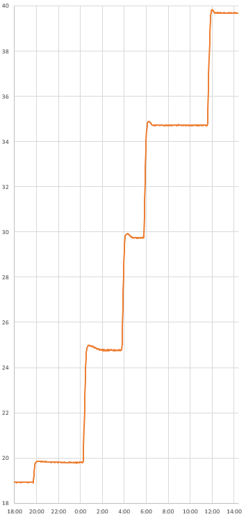
The result:
The Si7051 sensors we were using here have a maximum accuracy of ±0.1 °C in the human body temperature range of 35.8 °C to 41 °C, but this widens to ±0.25 °C between -40 and +125 °C. Even with this batch starting within spec the normalization tightens that band to about 0.05°C :
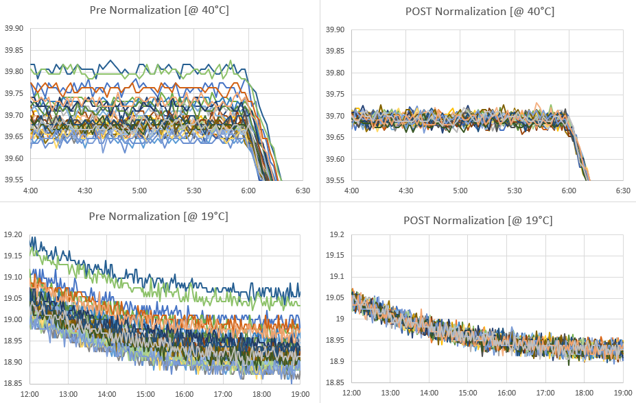
Like calibration, the raw data used to normalize sensors should cover the same range you expect to monitor in the field. There is no guarantee that fitting your sensors to an average will do anything to improve accuracy. However, sensors purchased from different vendors, at different times, tend to have randomly distributed offsets. In that case normalization also improves accuracy, but the only way to know if that has happened is to validate against some external reference. The method described here only corrects differences in Offset [with the B value] & Gain/Sensitivity [the M value]. Most temp sensors have a U-shaped error/noise distributions around their maximum accuracy point and if you see that pattern in the residual plots it means a linear correction is not sufficient and you might need to use a quadratic. Applying a linear correction to only one side of that curve (which I’ve done here) will increase errors on the other side of the distribution but as long as those amplified errors happen outside of the range of temperatures I intend to monitor the trade-off is acceptable.
Comments:
After the normalization of the Si7051 reference sensors, data from that same run was also used to calibrate the NTC sensors on those newly built loggers. Instead of using the cooling curve, the NTC calibration is done with a couple of the flat plateaus and physical ice-points collected separately. Being able to graph the large group with data from the same circulation bath makes is easy to identify & fix any copy/paste errors made during the calculations.
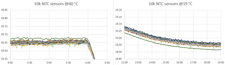
It’s interesting that the NTC’s clustered with an offset of ~0.05°C below the normalized Si7051s reference sensors. I’m attributing this shift to calculating the Steinhart-Hart equation constants with a data pair down at 0°C that was not in the normalization data set.
Out of forty DIY sensors, one (green) outlier above exhibited a slight nonlinearity problem that pushes it above the group at 40°C, but below the group at 19°C. Another exhibited a dramatic step-change behavior throughout the run and this logger will be rejected entirely from temperature sensing. Because our timing based method for reading NTCs treats the entire logger as a system, it will take more testing to see if this problem is with the physical sensor or with the ProMini module.
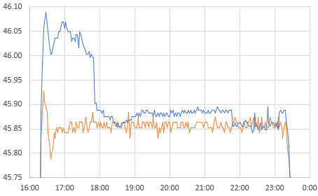
The higher resolution of the NTCs allowing us to look more closely at the Anova’s PID performance:
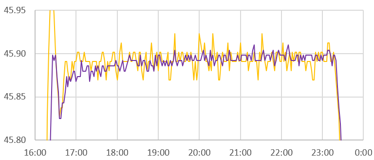
I suspect the 16 litre volume being driven here is near the practical limit of the little cookers capability, but the single wobble at the start of each plateau indicates a decent level of control. Especially considering the used cooker was $35 on eBay and the cooler was $10 at our local Goodwill. I’m still scratching my head about why the little Si7051 sensor modules read rising thermal spikes faster than the NTC but changes in the cooling direction stay aligned. I suspect this is due to direct conduction away from the NTC into the larger thermal mass of the ProMini board its attached to. Even with a thin housing that is IR transmissive, its not unusual to see a 15-20 minute lag in the NTC temperature readings relative to ambient.
References & Links:
Identifying Specific Problems Using Residual Plots
PID Controller – MATLAB (Guide) by Mike Deffenbaugh
PID Temperature Controllers: TUTCO Conductive
Anova’s Step-by-Step Guide to Building a Sous Vide Cooler
Considerations for water baths as calibration equipment
Guide on Secondary Thermometry: White et Al (2014)
Transition Temperatures of the Hydrates of Na2SO4…in Biomedical Thermometry
Calibration of TAO array of moored buoys: NOAA
Normalization applied to a group of Pressure Sensors