Tag Archives: promini

How to calibrate NTC thermistors (A DIY method you can do at home)

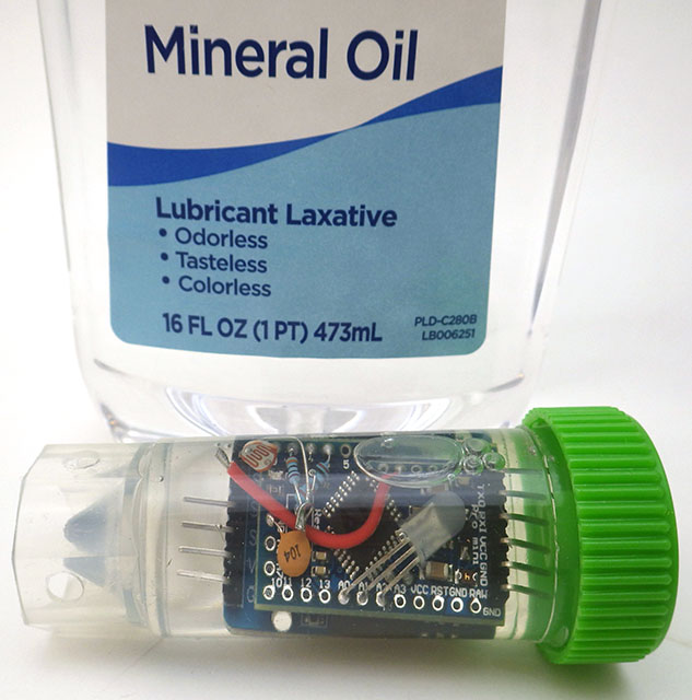
This post describes a thermistor calibration achievable by people who don’t have access to lab equipment with an accuracy better than ±0.15°C. This method is particularly suitable for the 10k NTC on our 2-module data logger handling them in a way that is easy to standardize for batch processing (ie: at the classroom scale). We use brackets to keep the loggers completely submerged because the thermal conductivity of the water around the housing is required or the two sensors would diverge. The target range of 0° to 40°C used here covers moderate environments including the underwater and underground locations we typically deploy into. This method is unique in that we use a freezing process rather than melting ice for the 0°C data point.

Use stainless steel washers in your hold-downs to avoid contamination of the distilled water and provide nucleation points to limit super-cooling. Before creating this bracket we simply used zip-ties to hold the washer weights.

Reading a thermistor with digital pins uses less power, and gives you the resistance of the NTC directly from the ratio of two Interrupt Capture Unit times. Resolution is not set by the bit depth of your ADC, but by the size of the reservoir capacitor: a small ceramic 0.1µF [104] delivers about 0.01°C with jitter in the main system clock imposing a second limit on resolution at nearly the same point. Large reservoir capacitors increase resolution and reduce noise but take more time and use more power. The calibration procedure described in this post will work no matter what method you use to read your NTC thermistor.

The I2C reference sensor is connected temporarily during the calibration via Dupont headers. Always give your reference sensors serial numbers so that you can normalize them before doing the thermistor calibrations.

Off-the-shelf sensors can be used as ‘good enough’ reference thermometers provided you keep in mind that most accuracy specifications follow a U-shaped curve around a sweet spot that’s been chosen for a particular application. The Si7051 used here has been optimized for the medical market, so it has ±0.1° accuracy from 35.8 to 41° Celsius, but that falls to ±0.13° at room temperatures and only ±0.25° at the ice point. If you use some other reference sensor (like the MAX30205 or the TSYS01) make sure it’s datasheet specifies how the accuracy changes over the temperature range you are targeting with the calibration.

The shortened Steinhart–Hart equation used here is not considered sufficiently accurate for bench-top instruments which often use a four or five term polynomial. However in ‘The Guide on Secondary Thermometry‘ by White et. al. (2014) the three-term equation is expected to produced interpolation errors of about 0.0025°C over a range from 0 to 50°C, and that is acceptable for most monitoring. To calculate the three equation constants you need to collect three temperature & resistance data pairs which can be entered into the online calculator at SRS or processed with a spreadsheet.

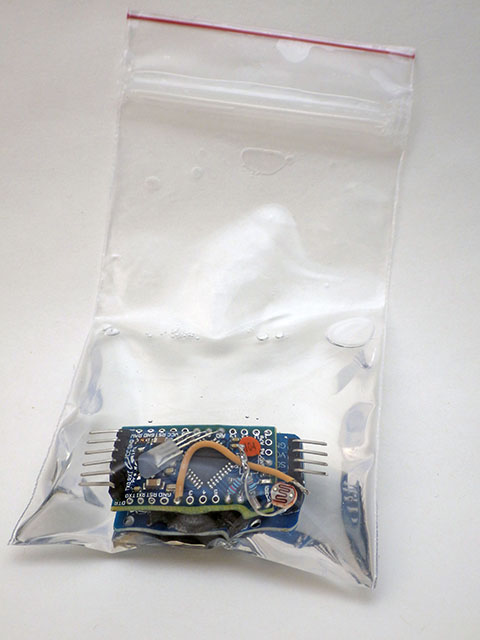
While these technical sources of error limit the accuracy you can achieve with this method, issues like thermal lag in the physical system and your overall technique are more important. In general, you want each step of the calibration process to occur as slowly as possible. If the data from a run doesn’t look the way you were expecting – then do the procedure over again until those curves are well behaved and smooth. Make sure the loggers stay dry during the calibration – switching to spare dry housing tubes between the baths: Moisture is the greatest cause of failure in sensors and humidity/water always lowers the resistance of thermistors. If in doubt, let everything dry for 24 hours before re-doing a calibration.

Data Point #1: The freezing point of water

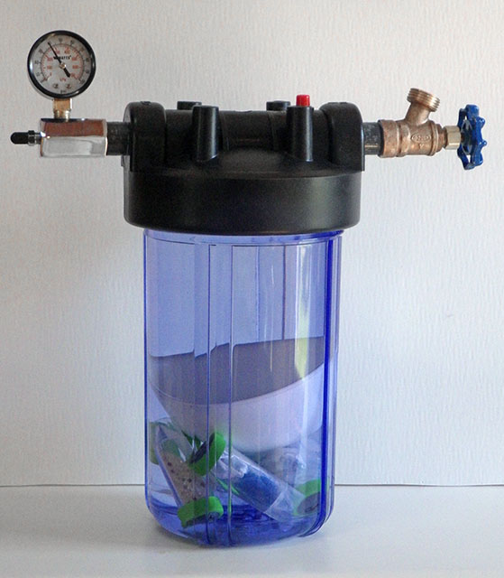
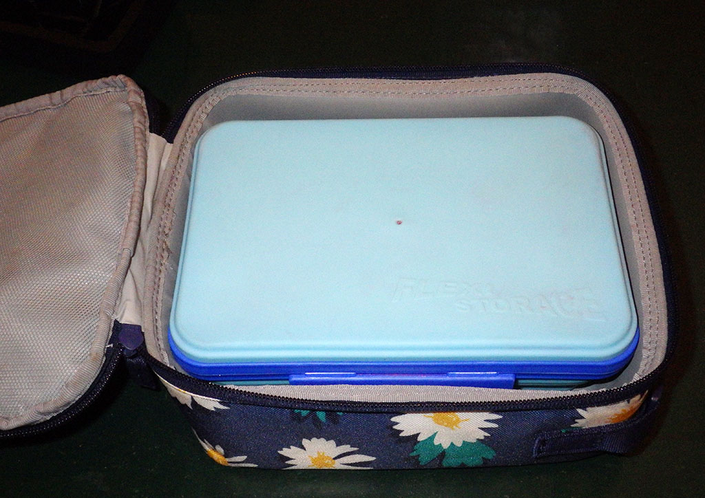
The most common method of obtaining a 0°C reference is to place the sensor into an insulated bucket of stirred ice slurry that plateaus as the ice melts. This is fine for waterproof sensors on the end of a cable but it is not easily done with sensors mounted directly on a PCB. So we immerse the loggers in collapsible 1200ml silicone food containers filled with distilled water. This is placed inside of a well insulated lunch box and the combined assembly is left in the freezer overnight, reading every 30 seconds.

Weighted holders keep each logger completely immersed. Soft-walled silicone containers expand to accommodate any volume change as the water freezes. This prevents the centrifuge tube housings from being subjected to pressure as the ice forms. **Position the loggers so that they are NOT in direct contact with the sides or the lid of the silicone container**.

The outer box provides insulation to slow down the freezing process. After testing several brands it was found that the Land’s End EZ wipe (9″x8″x4″) and Pottery Barn Kids Mackenzie Classic lunch boxes provided the best thermal insulation because they have no seams on the solid molded foam interior which also doesn’t absorb water spilled while moving the containers around.

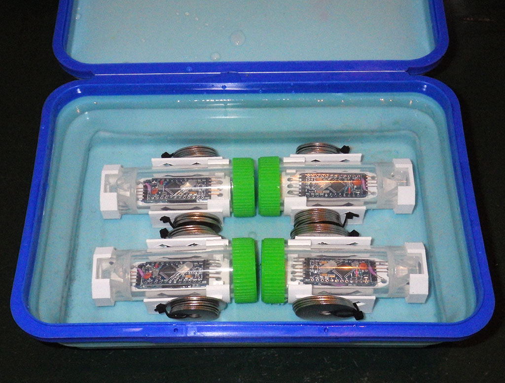
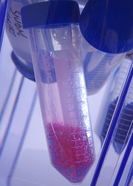
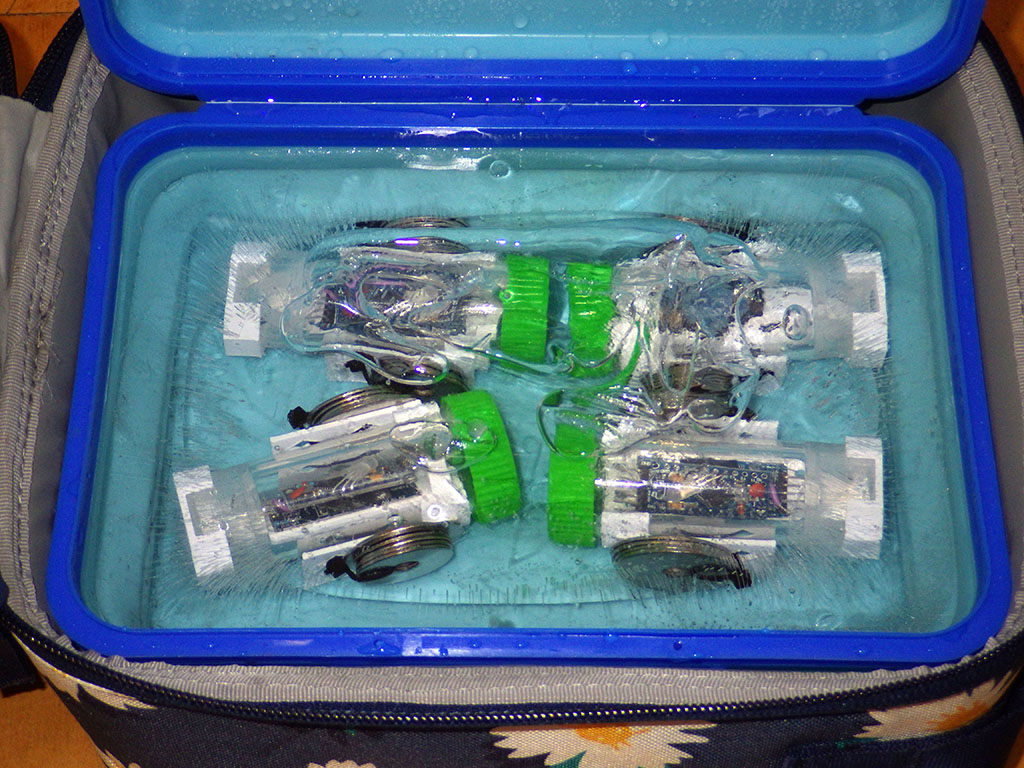
For the purpose of this calibration (at ambient pressure) we can treat the freezing point of pure water as a physical constant. So no reference sensor is needed on the logger while you collect the 0°C data. Leave the lunch box in the freezer just long enough for a rind of ice to form around the outer edges while the main volume of water surrounding the loggers remains liquid. I left the set in this photo a bit too long as that outer ice rind is much thicker than it needed to be for the data collection. Do not let the water freeze completely solid (!) as this will subject the loggers to stress that may crack the tubes and let water in to ruin your loggers.

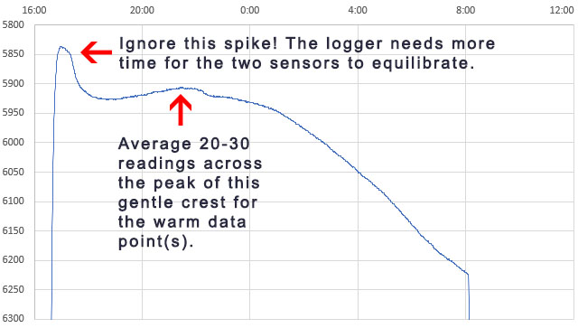
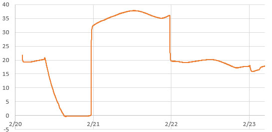
The larger bubbles in this photo were not present during the freeze, but were created by moving the container around afterward for the photo.

The trick is recognizing which data represents the true freezing point of water. Distilled water super-cools by several degrees, and then rises to 0°C for a brief period after ice nucleation because the phase change releases 80 calories per gram while the specific heat capacity of water is only one calorie, per degree, per gram. So freezing at the outer edges warms the rest of the liquid – but this process is inherently self-limiting which gives you a plateau at exactly 0°C after the rise:

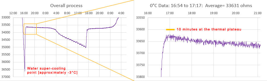
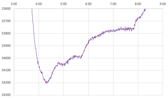
**NTC (ohms) gathered during the freeze/thaw process** graphed with the y axis is inverted because of the negative coefficient. The warm temperature data has been removed from the graphs above to display only the relevant cold-temperature data. Only the 10-20 minutes of data immediately after the rise from a super cooled state is relevant to the calibration. Cooling the insulated chamber from its room temperature starting point to the supercooling spike shown above took 7-8 hours.

Depending on the strength of your freezer, and the quality of the outer insulating container, the ice-point may only last a few minutes before temperatures start to fall again. An average of the NTC readings from that SHORT plateau immediately after the supercooling ends is your 0°C calibration point. This is usually around 33000 ohms for a 10k 3950 thermistor. Only the data immediately after super cooling ends is relevant and the box can be removed from the freezer any time after that event. I left the example shown above in the freezer too long but you have a reasonable window of time to avoid this. Once the freeze process initiates, it usually takes about 8 hours for the entire volume to freeze solid – after which you can see the compressor cycling as the now solid block cools below 0°C. You want to pull the sensors out of the freezer before that solid stair-step phase (at 8:00 above) if possible.

If the supercooling spike is not obvious in your data then change your physical configuration to slow the cooling process until it appears. You want the inner surface of your silicone container to have smooth edges, as sharp corners may nucleate the ice at 0°C, preventing the supercooling spike from happening. Use as much distilled water as the container will safely hold -the loggers should be surrounded by water on all sides.

In this image a freezer compressor cycle happened during post supercooling rise making it hard to see where the plateau occurred. This run was re-done to get better data.

Most refrigerators cycle based on how often the door is opened and those cycles can overprint your data making it hard to interpret. If you put a room-temperature box of water in the freezer between 6-7pm, it usually reaches the supercooling point around 2am, reducing the chances that someone will open the refrigerator/freezer door at the critical time. Even then, unexpected thermal excursions may happen if the freezer goes into a defrost cycle or an automatic ice-maker kicks in during the run. The time to reach that supercooling event can be reduced by pre-cooling the distilled water to ~5°C in the refrigerator before the freezer run. If any of the points on your curves are ambiguous, then do that run again, making sure the water is completely ice free at the start.

As a technical aside, the energy released (or absorbed) during the phase change of water is so much larger than its typical thermal content that water based heat pumps can multiply their output significantly by making slushies.

Data Point #2: Near 40°C

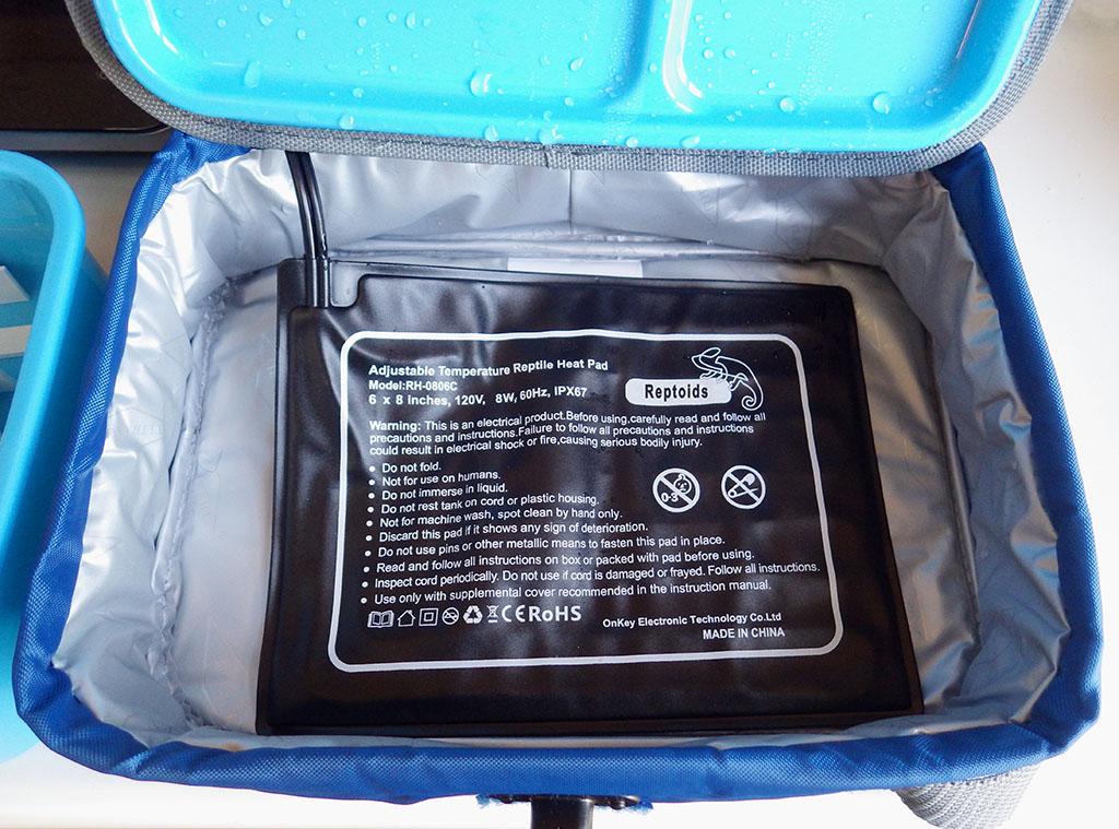
We have used the boiling point of water for calibration in the past, but the centrifuge tube housings would soften considerably at those temperatures. Ideally you want to bracket your data with equally spaced calibration points and 100°C is too far from the environmental conditions we are targeting. Heated water baths can be found on eBay for about $50, but my initial tests with a Fisher Scientific IsoTemp revealed thermal cycling that was far too aggressive to use for calibration – even with a circulation pump and many layers of added insulation. So we created an inexpensive DIY version made with an Arctic Zone Zipperless Coldloc hard-shell lunch box and a 4×6 inch reptile heating mat (8 watt). Unlike the ice point which must be done with distilled water, ordinary tap water can be used to collect the two warm temperature data pairs.

These hard-sided Arctic Zone lunch boxes can often be obtained for a few dollars at local charity shops or on eBay.

Place the 8-watt heating pad under the hard shell of the lunch box. **At 100% power** this tiny heater takes ~24 hours to bring the bath up to ~38°C. The **bath temp is relatively stable since the heater does not cycle**, but it does experience a slow drift based on losses to the environment. These heating pads sell for less than $15 on Amazon.

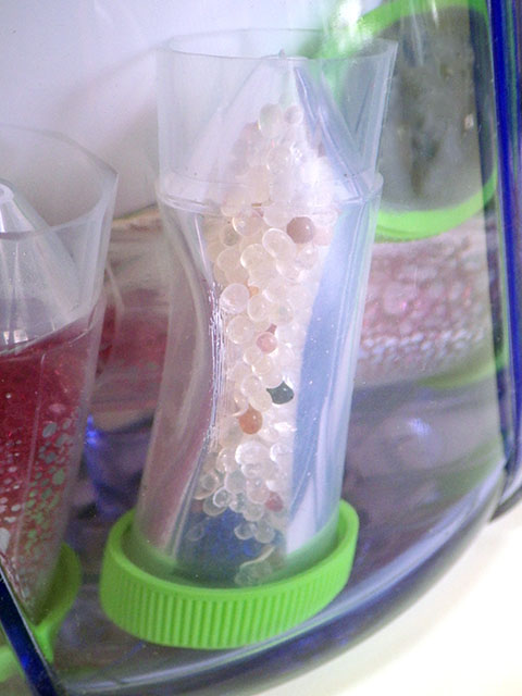
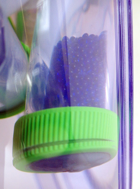
To record the temperature inside each logger, an Si7051 breakout module (from Closed Cube) is attached to the logger. A hold down of some kind must keep the logger completely submerged for the duration of the calibration. If a logger floats to the surface then air within the housing can thermally stratify and the two sensors will diverge. That data is not usable for calibration so the run must be done again with that logger.

The reference sensor needs to be as close to the NTC sensor as possible within the housing – preferably with the chip directly over top and facing the NTC thermistor.

Data Point #3: Room Temperature

The loggers stay in the heated bath for a minimum of 4 hours, but preferably 8 -12 hours. The idea is you want the whole assembly to have enough time to equilibrate. Then they are transferred to an unheated water-filled container (in this case a second Arctic Zone lunch box) where they run at ambient temperatures for another 8 -12 hours. This provides the final reference data pair:

**Si7051 temperature** readings inside a logger at a 30 second sampling interval. The logger was transferred between the two baths at 8am. Both baths are affected by the temperature changes in the external environment.

**Detail:** Warm temp. NTC ohms (y-axis inverted)

**Detail:** Room temp. NTC ohms (y-axis inverted)

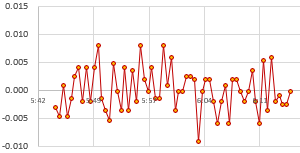
As the environment around the box changes, losses through the insulation create gentle crests or troughs where the lag difference between the sensors will change sign. So averaging several readings across those inflection points cancels out any lag error between the reference sensor and the NTC. Take care that you average exactly the same set of readings from both the Si7051 and from the NTC. At this point you should have three Temperature / Resistance data pairs that can be entered into the SRS online calculator to calculate the equation constants ->

I generally use six digits from the reference pairs, which is one more than I’d trust in the temperature output later. I also record the Beta constants for live screen output because that low accuracy calculation takes less time on limited processors like the 328p.

The final step is to use those constants to calculate the temperature from the NTC data with:
Temperature °C = 1/(A+(B*LN(ohms))+(C*(LN(ohms))^3))-273.15

Then graph the calculated temperatures from the NTC calibration readings over top of the reference sensor temperatures. Provided the loggers were completely immersed in the water bath, flatter areas of the two curves should overlap one another precisely. However, the two plots will diverge when the temperature is changing rapidly because the NTC exhibits more thermal lag than the Si7051. This is because the NTC is located near the thermal mass of the ProMini circuit board.

**Si reference & NTC calculated temperatures:** If your calibration has gone well, the curves should be nearly identical as shown above. With exceptions only in areas where the temperature was changing rapidly and the two sensors got out of sync because of different thermal lags.

Also note that the hot and warm bath data points can be collected with separate runs. In fact, you could recapture any individual data pair and recalculate the equation constants with two older ones any time you suspect a run did not go smoothly. Add the constants to all of the data column headers, and record them in a google doc with the three reference pairs and the date of the calibration.

Validation

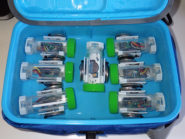
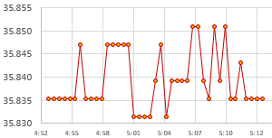
You should always do a final test to validate your calibrations, because even when the data is good it’s easy to make a typo somewhere in the process. Here, a set of nine calibrated NTC loggers are run together for a few days in a gently circulating water bath at ambient temperature –>

Two from this set are a bit high and could be recalibrated, but all of the NTC temperature readings now fall within a 0.1°C band. This is a decent result from a method you can do without laboratory grade equipment, and the sensors could be brought even closer together by using this validation data to normalize the set.

Comments

The method described above uses equipment small enough to be portable, allowing easy classroom setup/takedown. More importantly this also enables the re-calibration of loggers in the field if you have access to a freezer. This makes it possible to re-run the calibrations and then apply compensation techniques to correct for sensor drift. Validating calibration before and after each deployment is particularly important with DIY equipment to address questions about data quality at publication. Glass encapsulated NTC thermistors drift up to 0.02 °C per year near room temperatures, while epoxy coated sensors can drift up to 10x that.

At the ice-point, our resolution is ~0.0025°C but our time-based readings vary by ±0.0075°C. This is due to timing jitter in the ProMini oscillator and in the interrupt handling by a 328p. So with a [104] reservoir capacitor in the timing circuit, our precision at 0°C is 0.015°C.

Having a physical constant in the calibration data is important because most of the affordable reference sensors in the Arduino landscape were designed for applications like healthcare, hvac, etc. So they are usually designed minimize error in warmer target ranges, while getting progressively worse as you approach 0°C. But accuracy at those lower temperatures is important for environmental monitoring in temperate climates. The method described in this post could also be used to calibrate commercial temperature sensors if they are waterproof.

Calibrating the onboard thermistor a good idea even if you plan to add a dedicated temperature sensor because you always have to do some kind of burn-in testing on a newly built logger – so you might as well do something productive with that time. I generally record as much data as possible during the calibration to fill more memory and flag potentially bad areas in the EEprom. (Note: Our code on GitHub allows only 1,2,4,8, or 16 bytes per record to align with page boundaries) . And always look at the battery record during the calibration as it’s often your first clue that a DIY logger might not be performing as expected. It’s also worth mentioning that if you also save the RTC temperatures as you gather the NTC calibration data, this procedure gives you enough information to calibrate that register as well. The resolution is only 0.25°C, but it does give you a way to check if your ‘good’ temperature sensors are drifting because the DS3231 tends to be quite stable.

While the timing jitter does not change, non-linearity of the NTC resistance reduces the resolution to 0.005°C. Precision at 35°C also suffers, falling to 0.02°C. Using a 10x larger [105] reservoir cap would get us back to resolution we had at 0°C, as would oversampling which actually requires this kind of noise for the method to work. Either of those changes would draw proportionally more power from the coincell for each read so its a tradeoff that might not be worth making when you consider sensor lag.

For any sensor calibration the reference points should span the range you hope to collect later in the field. To extend this procedure for colder climates you could replace the ice point with the freezing point of Galinstan (-20°C) although a domestic freezer will struggle to reach that. If you need a high point above 40°C, you can use a stronger heat source. Using two of those 8 watt pads in one hard sided lunch box requires some non-optimal bending at the sides, but it does boost the bath temp to about 50°C. 3D printed PLA hold-downs will start to soften at higher temps so you may need to alter the design to prevent the loggers from popping out during the run.

If your NTC data is so noisy you can’t see where to draw an average, check the stability of your regulator because any noise on the rail will affect the Schmitt trigger thresholds used by our ICU/timer method. This isn’t an issue running from a battery, but even bench supplies can give you noise related grief if you’ve ended up with some kind of ground loop. You could also try oversampling, or a leaky integrator to smooth the data – but be careful to apply those techniques to both the reference and the NTC in exactly the same way because they introduce significant lag. Temperature maximums are underestimated and temperature minimums are overestimated by any factor that introduces lag into the system. In general, you want to do as little processing to raw sensor readings as possible at capture time because code-based techniques usually require some prior knowledge of the data range & variation before they can be used safely. Also note that our digital pin ICU based method for reading resistors does not work well with temperature compensated system oscillators because that compensation circuitry could kick in between the reference resistor and NTC readings.

And finally, the procedure described here is not ‘normalization’, which people sometimes confuse with calibration. In fact, it’s a good idea to huddle-test your sensors in a circulating water bath after calibration to bring a set closer together even though that may not improve accuracy. Creating post-calibration y=Mx+B correction constants is especially useful for sensors deployed along a transect, or when monitoring systems that are driven by relative deltas rather than by absolute temperatures. Other types of sensors like pressure or humidity have so much variation from the factory that they almost always need to be normalized before deployment – even on commercial loggers.

Normalize your set of reference sensors to each other before you start using them to calibrate NTC sensors.

References & Links:

SRS Online Thermistor Constant Calculator
Steinheart & Heart spreadsheet from CAS
S&H Co-efficient calculator from Inside Gadgets
Molex Experimenting with Thermistors Design Challenge
Thermistor Calibration & the Steinhart-Hart Equation WhitePaper from Newport
ITS-90 calibrates w Mercury(-38.83), Water(0.01) & Gallium(29.76) Triple Point cells
Guide on Secondary Thermistor Thermometry, White et al. (2014)
Steinhart-Hart Equation Errors BAPI Application Note Nov 11, 2015
The e360: A DIY Classroom Data Logger for Science
How to make Resistive Sensor Readings with DIGITAL I/O pins
Single Diode Temperature Sensors
Measuring Temperature with two clocks
How to Normalize a Set of Sensors

A DIY Pressure Chamber to Test Underwater Housings

Pressure testing has been on the to-do list for ages, but the rating on the PVC parts in our older housings meant we weren’t likely to have any issues. However, the new two-part mini-loggers fit inside a thin walled falcon tube, which raised the question of how to test them. There are a few hyperbaric test chamber tutorials floating around the web, and we made use of one built from a scuba tank back at the start of the project, but I wanted something a less beefy, and easier to cobble together from hardware store parts. Fortunately Brian Davis, a fellow maker & educator, sent a photo of an old water filter housing he’d salvaged for use with projects that needed pressure tests. Residential water supply ranges from 45 to 80 psi so could replicate conditions down to 55m. That’s good for most of our deployments and certainly farther than I was expecting those little centrifuge tubes to go.

This mini pressure chamber was made from a Geekpure 4.5″x10″ water filter housing, 2x male-male couplers, a garden tap, & a pressure gauge with a bicycle pump inlet. (~$70 for this combination) The relief valve & o-ring required silicone grease to maintain pressure.

I first tested 50mL ‘Nunc’ tubes from Thermo. These are spec’d to 14psi/1atm, but that’s a rating under tension from the inside. I put indicator desiccant into each tube so small/slow leaks would be easy to see and used a small bicycle pump to increase the pressure by 5psi per day. These tubes started failing at 25psi, with 100% failure just over 30psi. Multiple small stress fractures occurred before the final longitudinal crack which produced an audible ‘pop’ – often four or more hours after the last pressure increase. If 20psi is the max ‘safe’ depth for these tubes then the 50mL tubes can deployed to about 10m with some safety margin for tides, etc. This result matches our experience with these tubes as we often use them to gab water samples while diving.

As expected, the self-standing 30mL tubes proved significantly more resistant. All of them made it to 45psi and then progressed through various amounts of bending/cracking up to 100% failure at 55psi. Where the caps were reinforced (by JB weld potting a sensor module) the rim threads of the cap sometimes split before the tube itself collapsed:

Silicone grease was added to some of the caps although none of the dry ones leaked before the bodies cracked.

So the 30mL tubes have a deployment range to 25m with a good safety margin. The plastic of these tubes was somewhat more flexible with some crushing almost flat without leaks. This implies we might be able take these a little deeper with an internal reinforcement ring (?)

The next experiment was to try filling the tubes with mineral oil to see how much range extension that provides:

A third logger was submerged using only a sample bag:

The bag was included to test the ‘naked’ DS3231 & 328p chips. We’ve had IC sensors fail under pressure before (even when potted in epoxy ) Although it’s possible the encapsulation itself was converting the pressure into other torsional forces that wouldn’t have occurred if the pressure was equally distributed.

Again we moved in 5 psi increments up to 80 psi – which is the limit of what I can generate with my little bicycle pump. At 50psi some mineral oil seeped from the bag and at 70psi the ~1cm of air I’d left in the 50mL tube caused similar leakage. On future tests I will spend more time to get rid of all the bubbles before sealing the housings.

At 70psi the 50mL tube dented & sank and the lid started seeping oil (but did not crack)

The loggers continued blinking away for several days at 70, 75 & 80psi, but eventually curiosity got the best of me so I terminated the run. We were also getting uncomfortably close to the 90psi maximum test pressure on that polycarbonate filter housing. I was hoping to have some weird artifacts to spice up this post but no matter how hard I squint there really were no noticeable effects in the data at any of the pressure transitions – basically nothing interesting happened. I thought the resistive sensors would be affected but the RTC & NTC temperature logs have no divergence. The LDR looks exactly like a normal LDR record with no changes to the max/mins outside of normal variation. The battery curves are smooth and essentially indistinguishable from ‘dry’ bookshelf tests on the same cells. But I guess in this kind of experiment success is supposed to be boring… right? With mineral oil these little guys can go anywhere I can dive them to – even if the ‘housing’ is little more than a plastic bag.

One thing of note did happen after I removed the loggers from the chamber: I accidentally dropped the 30ml logger on the counter while retrieving it from the chamber and a thin white wisp of ‘something’ started swirling around the clear fluid inside the logger. This developed slowly and my first guess was that the capacitor had cracked and was leaking (?)

By the time I managed to capture this photo, the fine ‘smoke’ seen earlier had coalesced into a larger foam of decompression bubbles.

After emptying that oil, the logger itself went into a red D13 flashing BOD loop for a while but by the time I’d cleaned it up enough to check the rail, the battery had returned to it’s nominal 3v. My theory is a similar off-gassing event was happening inside the battery – briefly causing a droop below the 2.7v BOD threshold. So it’s possible that while the loggers are not depth limited per se using mineral oil, components like the separator in a battery may still be vulnerable to ‘rate-of-change’ damage. After more than two weeks at depth, I had vented the chamber in less than a minute. Of course when retrieving loggers in the real world I’d have to do my own safety stops, so this hazard may only affect loggers that get deployed/retrieved on a drop line.

I’ll run these loggers on the bookshelf for a while to see if any other odd behaviors develop. After that it will be interesting to see how well I can clean them in a bath of isopropyl (?) as I suspect that the mineral oil penetrated deep into those circuit board layers.

Addendum: 2023-05-30

Although the units sleep current was the same as before the pressure testing, the battery in the 30mL tube barely made another twelve hours on the bookshelf before the voltage dropped again – well before the expected remaining run time. So it’s a safe bet that any deployment which exposes coin cells to pressure at depth is a one-shot run. Given how cheap these batteries are, that’s pretty much a given when deploying these little loggers even if they remain dry.

Addendum: 2023-12-01

Short 30ml tubes work well for single-sensor applications, but classroom labs needed to switch between different sensor modules easily. So we added 3D printed rails holding mini breadboards to provide this flexibility, and the 50mL centrifuge tubes provide the space for these additions. They may not have the same depth range, but they are robust enough for most student experiments.

It’s also worth noting that these tests were done with the standard ‘plug-style’ caps that come with the NUNC 50ml centrifuge tubes. A few companies make tubes with an O-ring integrated into the cap (made of silicone or ethylene propylene) which gets compressed when the threads are tightened. Those would provide another layer of moisture resistance at that seal, although they wouldn’t do much to prevent the crush-failures. Unfortunately the Nalgene Oak Ridge high-speed polycarbonate centrifuge tubes that could resist those forces have necks pinched-in to a diameter too small for the modules in our logger.