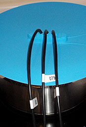
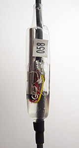
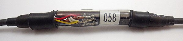
Give each sensor a serial number, but don’t label the sensor itself as I have in this photo or the labels will just fall off during the steam point testing. After adding crimp pins to the wire ends it becomes easy to gang them together on a breadboard for testing. Despite Maxim’s warnings, I had star configurations above 20 sensors reading well with them close together like this.

I’m probably not the first person to note that sensor calibration is one of the big differences between the mountains of data coming from the citizen science movement and that produced by research professionals. (…mea culpa…) After opening this can of worms, I think I am beginning to understand why: Accuracy calibration rapidly gets complicated, or expensive, and often it’s both at the same time. By the time you have what you need to do the job, the difference between a $0.30 sensor, and a $30 sensor, is pretty insignificant. So it’s no surprise that few people work on calibration methods for low cost sensors, or why normalization approaches are used instead.

But I am already spending far too much on this little hobby, so despite knowing that the folks over at Leighton Telescope managed to get their DS18b20’s to about ±0.01°C with a NIST traceable thermometer, I thought I would see how far I could get on my own.  I suppose if I was an alpha geek,  I would make my own platinum RTD  and calibrate the sensors against that.  But I’m not quite there yet. I should also point out that numbers are not my strong suit, so there could be some significant errors in what I have cobbled together here and I appreciate any feedback to help correct those…

The first thing that occurs to me is: Can you read the temperature more accurately  by averaging a bunch of these sensors together?  If the readings from the sensors have a mean and standard deviation, then as the number of sensors increases then the standard deviation should decrease…right?  The data sheet gives you a sense of how far you can get with that approach, because I assume that Maxim/Dallas used a very large number of sensors to derive their typical performance curve:

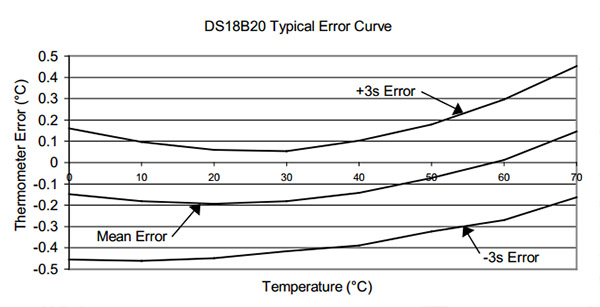
But if I understand what people say about this graph, the only reason the 3 sigma spread on that graph looks better than ±0.5 at 20°C is because the errors in the sensors used to derive that curve were truly random, and had a nice Gaussian distribution around that mean. However, since the actual batch of sensors I am holding in my hand is likely from the same production run, it is subject to systematic errors that don’t cancel each other out so nicely. And since I bought them on eBay, there is also a chance that they might be fake DS18b20’s.  So I could have no idea how my mean error line was related to the one on Maxim’s graph.

But there are still useful things you can do with this kind of averaging:

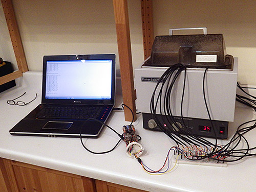
The front temperature display on this clunky old Fischer Scientific was off by more than 2°C, and it was missing a foot. While it’s hardly a temperature chamber,  the insulation and covering lid produced a slow cooling curve, so I could be reasonably confident the sensors were being exposed to the same temperatures. Don’t use data from the rapid heating cycle, because temperatures are likely to be unevenly distributed in the bath.

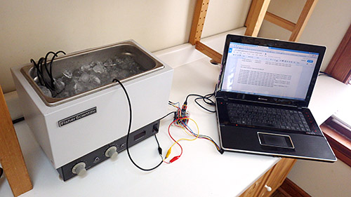
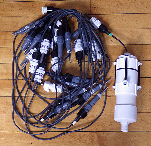
First of all you can get rid of the bad sensors by selecting a group that has a consistent behavior over the temperature range you are looking at, with readings that fall within the manufacturer’s specifications.  To get enough data for this kind of assessment, I needed to run at least 10 sensors at the same time so that the average had some statistical weight. For this testing I picked up an old five Litre isotemp bath (you can find them for $25-$50 on eBay) but you could just as easily do this with hot water in a styrofoam cooler. With about 20 sensors on a breadboard in a star configuration (4.7k pullup), I brought the water bath up to a stable 40°C, and then moved the entire thing out into the fridge and left it logging during the cool down. The lid was on, and I had several towels over top to make the process go as slowly as possible.  It took 12 to 24 hours for each batch of sensors to reach ~5°C.

With this data in hand, I looked at the residuals by subtracting each sensors raw reading from the average of all the sensor readings.  This exercise sent one DS18 straight into the bin, as it was more than 2.5°C away from the rest of the herd for its entire record.  Another was triaged due to a strange “hockey stick” bend in it’s residual around 25°C.  I threw out the data from those two duds, and recalculated the average & residuals again.  Just to be on the safe side I decided not to epoxy any sensors into a long chain if they were more than 0.3°C away from the average. (although I am still wondering whether eyeballing residuals like this is enough to exclude the right outliers?)

You can then normalize the sensors to each other by fitting a quadratic equation to a graph of each sensor & the overall average line. Excel can generate these coefficients for you with the linest function, or it can solve the quadratic with Goal Seek.  But the easiest method I found was make a 2nd order (but not higher) fit with the chart tool’s trendline function. Make a scatter plot of the data with the averages on the Y axis, and data from one individual sensor on the X axis.  Then right click on the data points to select them, and choose ( Add Trendline ) from the pull down menu, with the [ ] Display equation on chart tick box checked.      (here is an example of the technique using an older version of Excel)

The equation you see displayed will convert that particular sensors output into corresponding temperatures on the average line. With this transformation, each sensor will yield the same reading if it is in the same thermal environment, and you can accept that any differences between two sensors in the chain represent real differences in temperature.

This kind of normalization is as far as most people go. However for the reasons I outlined above, we can’t be sure that we were using a valid sample for that mean data. In my tests it looked like I did not have an equal distribution of sensors above and below the average line, so I still didn’t really have a handle on whether this was improving the absolute accuracy. (I will post some example graphs of this later…)

That brought me to calibrating the DS18b20’s against intrinsic physical standards which rely on the fact that during a phase change  (melting, freezing or boiling)  adding and removing heat causes no change in temperature. In fact those heating curve plateaus are known so precisely that they use them at NIST to calibrate the expensive thermometers that I am trying to avoid buying.  Today they do this with Gallium‘s triple point (29.7666 °C) and the triple point of water (0.010 °C), but they used to use Gallium’s melting point plateau. (29.7646 °C)  Gallium sells for less than a buck a gram on Amazon and a density of about five grams per cubic centimeter means a block big enough to surround one of the DS18’s is almost within a DIY’ers budget. (100 grams will make a disk about two inches across and a quarter inch thick) But considering that commercial Ga melt cells cost about three grand, either that stuff is nasty enough to get me into trouble, or you need allot more more of it, at higher purities than you can buy on eBay to build one.  Then there is the significant time it would take to refreeze the block again for every single sensor. And finally, all exposed metal must be carefully lacquered as Gallium will form an amalgam with many metals, and any dissolved metals will compromise the purity of the bath, shifting the melting point. And you would probably have to cover everything with Argon wine preserver.

So I went hunting for other substances I could use for a mid range calibration point and found several good boiling points such as: Ether (35 °C), Pentane (36.1°C), Acetone (56 °C), and Methanol (66 °C). Despite my enthusiasm over coffee the next morning,  all of them were summarily rejected by my wife, who strongly suggested that I look for calibration procedures that do not create large amounts of highly explosive vapor. Given how unstoppable she usually is in the pursuit of  good data, I was not expecting this outburst of common sense 🙂

So I looked at the other primary standard used to calibrate pt100’s. Turns out it is possible to make your own triple point cell, and if that’s not good enough for you,  Mr. Schmermund also produced plans for a freezing point of mercury cell (–34.8 °C) (See: “Calibrating with Cold”, Shawn Carlson, Scientific American, Dec. 2000 issue).  However the local 7-11 was fresh out of liquid nitrogen when I checked, and I had this gut feeling that risking mercury induced brain damage was not going to pass the cost/benefit analysis either. If I actually did need sub zero calibration I think I would try using Galinstan, (−19 °C) which is now replacing mercury in glass thermometers.

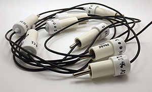
Pre-chilling the sensors in one corner of the bath makes the process much faster. Hold the sensors by the cable, not the metal sheath, or heat from your hands will affect the readings.

It was looking like calibrating against anything other than distilled water was going to take a substantial amount of effort compared to what I was seeing in the NIST and EPA videos. Most sources indicated that the ice point and steam points were at least an order of magnitude more accurate than my ±0.1°C target, making them suitable for the exercise.

While the overall procedure is pretty easy, it did help to practice a few times to get a sense of when I could trust the readings. Checking that you have just the right amount of water in your ice bath makes a big difference, and don’t run the sensors at full tilt or they will self heat. (I left 15 seconds between readings) Since errors on my part would cause the sensor to be warmer than the true ice point, I took the lowest reading, while stirring, as my final reading. The difference between stirring, and not stirring was usually 1-2 integer points on the sensors raw output (0.0625-0.13 C) and this was consistent for all the sensors.

If these sensors were linear then reading the ice point was a direct measure of the b in y=mx+b. And this got me wondering if one point calibration was enough all by itself.  But once again my wet blanket science adviser assured me that nothing on those graphs told me if the offset was constant over the sensors range. Hrmph! (Although according to Thermoworks, ice point alone can be a good way to check for drift, because the most common error in electronic temperature sensors is a shift in the base electrical value)

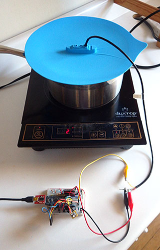
I found a silicone vegetable steamer lid for the calibration that had three DS18B20 sized holes in it already.  Getting the right pace for your slow rolling boil is important, and this lid sheds the condensed water back into the pot reasonably well. Alligator clips also help speed the process.

So I moved on to measuring the steam point. Water’s boiling point is not necessarily at 100°C and the only factor that is really involved in the variance is atmospheric pressure. Altitude is often given as an alternative when pressure information is not directly available and there are plenty of places to look up elevation and barometric pressure data (& converters) for the necessary corrections.

I already had some MS5805-02 sensors on hand, so with the help of Luke Millers library, I could read my local atmospheric pressure for the correction directly.  The accuracy of my pressure sensor was ±2.5 mbar (similar to  the more common BMP180) with the B.Pt adjustment equation being: Corrected B.Pt.=100 (°C)+((PressureReading-1013.25mbar)/30)  So the 5 mbar total error range in the pressure sensor could change the adjusted boiling point by up to 0.166°C.  This means that the error in my pressure sensor measurement is at least as significant as the other aspects of this procedure. Better than the default ±0.5°C, but it puts a limit on how accurate I will can get with my steam point measurement.

Cutting down the stacks on the Fred steamer lid allowed me to do multiple sensors at once. This saves time, but be careful or you will pay the piper with a few burned fingers when you change them out.

With each sensor just under the surface of the boiling water (since the evaporation process happens a little bit above 100°C) each one took about 5 minutes to warm up to reading temperature with the water on a slow to medium boil (and it was easy to see that on the serial monitor) I didn’t consider the test done till I saw at least a full minute of stable output (reading the sensor every 10 seconds) Since errors in my technique would produce readings on the cold side, I took the highest ‘frequently repeated’  number as the final reading. Most sensors settled nicely while some of them toggled back and forth by one integer point from one reading to the next.

In comparison to the steam point procedure, I trust the Ice point as more reproducible because it does not suffer from any pressure information dependency. Perhaps more important is the fact that 100°C is far away from my 20-30°C target range, leaving the possibility for significant errors if the sensors have a non-linearity problem.

With the ice and steam readings in hand, I could construct a two-point calibration for each of my DS18B20’s with slope M=Δy/Δx, and B=(the ice point reading).  (explained here, and that left you in the dust there are lots of fill-in-the-blank spreadsheet templates on the web)

At this point I am still doing tests & chewing on numbers, but the standard deviations around the mean line are being reduced by this ice&steam point calibration. The problem is that even after I apply the resulting slope and intercept I still have significant residuals from a mean that is derived with the corrected numbers. I thought that the two point calibration would make the graphs the individual sensors line up very closely with one another, and that they would have nearly identical slopes(?) I am left wondering if larger sensor errors up at 100°C mean that I need to apply some additional process to normalize my sensors to each other in the 30°C range after doing the two point calibration.  But using the process I described above would generate ‘b’ value corrections, and I am very reluctant to modify my y intercept numbers because I think using the ice point to measure that offset is robust. These doubts about accuracy of the steam point, the sensors linearity, and my lack of a nice “mid-range” standard to calibrate against, have me hunting for a method which would gracefully combine a single (ice) point calibration with normalization. And the dip in the datasheet’s mean error curve between 20-30°C implies that even after applying ice point corrections my average line will still be 0.05°C lower than actual (?)

Another important observation is that the means generated from the uncorrected data were within 0.14-0.16°C of the means calculated after applying the two point calibration. Either my sensors actually did have a reasonably normal distribution of error, or I might have missed something important.  The implication in that first case is that normalization alone should improve your overall accuracy, but I still need to get my hands on a calibrated pt100 to know for sure….Argh!

Addendum 2015-05-18

Bil Earl just posted a beautifully written article on sensor calibration, which puts everything here into context. A great job once again by the folks over at Adafruit!

Addendum 2016-02-12

Just adding a quick link to a small post on the pre-filtering I do with these sensors, which I only posted because no one else seems to bother posting data on the ‘typical quality’ you see with the cheep eBay sensors. And after splashing out on a Thermapen reference thermometer ($200), I can try a multi-point calibration for these sensors that is closer to my target temperature range.

Addendum 2016-03-05

Just put the finishing touches on a new calibration approach which, compared to this ice & steam point method, was an order of magnitude faster to do. If you are calibrating a large number of sensors, the reference thermometer is definitely worth the investment.

Temperature is a fundamental physical parameter which can be used to track how water moves and interacts with the rest of the environment. Most waterways in the world are multi use, and temperature sensors are a simple way to monitor rivers and streams, to see how they are being affected by urban pollution, agricultural runoff,  solar heating, groundwater exchange, etc.  In larger water bodies, we also want to track the cycles of temperature stratification.  Sometimes we deliberately disrupt thermoclines with aeration to preserve game fish, but at other times we depend on metalimnion stability to provide a barrier between the E. coli we dump in, and the water we take out for drinking.  Monitoring hydrothermal plumes can even shed light on geological activity under the ocean floor.

My first attempt with epoxy & lengths of 1/2″ pvc was successful enough to keep me going. For shallow water deployments, a simple treatment like this would probably be good enough to last for many months. Epoxy is the most expensive component, so each node cost ~ $4.00 with the benefit that each sensor is very robust afterward. You can also check out Luke Miller’s sensor waterproofing on his blog.

Temperature is also a key metric of ecological integrity because it exerts a profound influence on aquatic creatures. Many species time their reproduction and migration according to seasonal water temperatures and, as temperature increases, the capacity of water to hold dissolved oxygen is reduced. In coastal environments, temperature and salinity are very strongly associated so you can use it as a reliable proxy to record tidal cycles, and saline intrusion into fresh water habitats.

All of these applications require simultaneous sampling at different depths and locations, so arrays of temperature sensors are a standard tool for addressing water quality issues. Today, many researchers are looking to the open source movement to help make these large installations more affordable.  One obvious candidate is the inexpensive DS18b20 temperature sensor because it’s one wire protocol makes it possible to string them together in a daisy-chain configuration.  Electronics hobbyists have taken note, and are putting them all over the place with Cat5 network cables. Reading those pages convinced me to take a closer look at the DB’s from the perspective of the Cave Pearl Project: Would it be possible to turn these humble band-gap temperature sensors into something like a research quality thermistor string?

A review of typical commercial options gives you a sense of how much it actually costs to build a network of temperature sensors:

The iButtons are basically disposable, and I don’t think it would be worth anyone’s time to make them from scratch if all you need is 0.10±0.7°C.  But if you need more precise information, a simple 10 node string puts you around $1500 in the mid range, and $4000+ at the geotechnical high end.  Factory calibration of 0.0625 ±0.5°C puts the DS18B20s somewhere between the Hobo loggers and the low end Themochrons. But with each sensor on the same chain, you would be able to keep all the sensors synchronized better than stand alone units.  After seeing the elegant pro-level system, I knew I also wanted something that could be assembled from interchangeable segments, to customize the chain for each installation.

I googled and grazed my way through various YouTube videos, instructables, etc. looking at how others had water-proofed these sensors. After digesting that, I produced a some prototypes using a modified version of my underwater connector idea that have the DS18b20 potted in an irrigation pipe coupling:

~ $9 each for materials. The barbs are tapped to aid adhesion, JB Plasticweld forms a plug to hold the epoxy in.

The 1-Wire Address Finder and the library from Miles Burton work well with this changeable configuration. I preferred the code over at Paul Stoffregen’s site, as it gives you the raw integer reading, the ROM address, and the temp in °C as soon as you connect a new sensor.  But like most of the scripts that uses address arrays, it will read them in numerical, rather than physical order.  So you will eventually end up hard coding the Rom addresses unless you switch over to something like the DS28EA00 that supports sequence detection through a chain mode function. This allows you to discover the registration numbers according to the physical device location in a chain, and if the DS28 also had better resolution/accuracy than the dirt cheap DS18’s, I’d be converted.

The one-wire guide at the Arduino playground has a most valuable tip for driving a string of sensors like this:

“The master can address all devices on the bus simultaneously without sending any ROM code information. For example, the master can make all DS18B20s on the bus perform simultaneous temperature conversions by issuing a Skip ROM [CCh] command followed by a Convert T [44h] command.”

This means that I can minimize the number of times the Arduino has to wake-up for each set of readings. But these sensors are still going to pull about 1.5 mA each during the 750ms 12-bit conversions, so there is going to be a substantial power demand during each set of sensor readings even if I put the μC to sleep while it waits for the data. (and you can only sleep if you are not using parasite power) Thirty or more sensors on the bus will also generate allot of communication and data buffering. I have no idea yet how much juice all that is going to take so I built some larger housings, with room for twelve AA batteries, to drive these long daisy-chains:

This prototype is 14m long, with 1m, 0.5m and 0.25m cables.  I’ve had no data reading errors so far…

Maxim has guidelines for reliable long line 1-wire networks which suggests that longer networks need 100 Ω resistors at each node for distributed impedance matching or you could run into timing/reflection issues. As I am working in reasonably restricted cave environments where the floor to ceiling distances rarely exceed 20m, I did not add these resistors. If I start seeing the dreaded 85°C error after I load the bus, I will try a lower value pullup resistor, or perhaps a barrier diode. There is even an I2C to one wire bridge out there that can adjust the strength of the pull-up dynamically as your network grows, although since the one-wire bus is so easy to get running, I would only cobble the two networks together if I had an unusual situation.

I am using Deans 1241 Micro 4R plugs, which just barely fit inside the pipe. These connectors are really solid, but the trick is to get the wires to fold without pinching when you mate the o-ring to the seat on the opposite side of the connector.

The sharp eyed will note that there are four conductors on that interconnect.  I used four conductor cable for added strength because silicone jacket cables are so soft and floppy that the sheath really provides no support at all. And this offers the potential for a second one-wire network that is separate from the first if communication errors start to appear. Alternatively, I could add other one wire devices to that second line for more functionality. I have not figured out what this might be yet, but perhaps I could include some kind of leak detector to make the system more robust. I am also keeping an eye on the one-wire weather station crowd to see if an interesting sensor pops up there.  And finally, I wanted a four wire connector that could also be used with I2C breakouts, as most of my other builds use sensors with that protocol.

With 27 nodes, this is approaching the largest string I would want to deploy on a dive.  I need to put some thought into how to handle this massive tangle hazard safely.

I have replaced the cable that came with the “waterproof” DS18B20 sensors, as the insulation was far too thin for the rough handling I expect to see and the 28awg wires would add significant resistance over a long run.  But silicone jacket cable is expensive and I am still searching for an affordable 24awg, 4-conductor option. (If you have a suggestion, please pop it in the comments!)  The PVC and Poly-urethane jacket cables I have tried so far are just too stiff to “hang right” under water without a weight on the line, and this would put strain the data connections.  The standard solution is to run a suspension wire alongside the thermistor string with the data lines connected to this armored stiffener. While this works great off a boat or a buoy, I would prefer not to have to deal with those extra components on a cave dive.

After addressing the issues with the physical build, I still have an elephant standing in the corner.  While an accuracy of ±0.5°C might be good enough to track the refrigerator in the garage,  ±0.1 °C is about as coarse as you want to go for research applications. So a lot of the burden of making this thing really functional will be the calibration. If you replace the Arduino’s 10-bit ADC, then there are thermistors that give you ±0.1°C right out of the box, and I would like to get these DS18b20’s into that ball park before I say the newest addition to the Cave Pearl family is ready to deploy.

Maxim has a document describing how to curve fit the error of a band-gap based digital temperature sensor with 2nd order polynomials to achieve accuracies in the 0.02-0.04°C range,  but they make the assumption that you already have a NIST traceable platinum RTD to determine what the errors actually are. But what if you don’t have that $5-600 piece of kit just lying around? (+another $150/year for the required annual re-calibration) Is there any other way to calibrate temperature sensors like this to improve their accuracy?

Actually, there are verification procedures that use the ice and steam points of water, and I will detail my attempts to use these “old-school” calibration methods in the next post. In theory at least, these intrinsic standards can bring our DS18b20’s well within a mid-range accuracy target of  ±0.2°C.  At the end of it all I will try to borrow a certified pt100 to see how close I actually got.

Addendum 2015-02-23

After handling that long chain for a few days of calibration, I realized that I needed to mount those sensors with a much smaller physical profile or they were going to be a pain the backside under water. So I came up with a simple combination of heat shrink tubing and epoxy that keeps the sensor much closer to the cable than a hard-sided mould:

Using clear heat shrink will let me monitor leaks, aging, etc. There is heat shrink tubing on those solder joins, but it became invisible in the clear epoxy.

Heat from the bottom and as the tubing shrinks the epoxy “flows” up to the other end. When you seal the upper end leave some excess epoxy trapped in the tube. Apply another ring of shrink to cap it off, and with both ends fully sealed & cooled down, gently heat the entire surface. As the leftover wrinkles disappear the heat shrink tube turns into a tension structure creating a smooth rounded profile.

The trick is to seal one end of the clear tubing first, and then inject the epoxy into that from the open end.  Once the tube is about 2/3 full 0f epoxy, shrink the upper open end of the tubing down to it’s minimum diameter. Very gently heat several spots along the tube  – as those areas contract it pushes the epoxy up toward the open end.  Then wipe away any excess so the meniscus is level, and seal the upper end of the outer tube to the cable with a short section of adhesive lined heat shrink tubing, making sure that you trap as few bubbles as possible. I usually use adhesive lined heat shrink for those two end tubes, and I let the upper ring completely cool so that if forms a good seal before heating the rest of the clear heat shrink tube.  I usually use Loctite E-30CL  epoxy as this sets much more quickly after the reheating process, often becoming hard in about 30-45 minutes. This approach to mounting the sensors would also work with ‘naked’ Ds18b20’s, but having the sensors already mounted in the stainless steel sleeve makes it much easier to do the ice & steam point calibrations before you commit to actually using a particular sensor.  At only $1.50 each, you should expect to triage at least some of them for being out of spec.

Completely encasing the sensor like this will induce some thermal lag, if you are really worried about that you could make the tubing shorter and not seal the upper end, leaving the metal sleeve exposed.  If field handling indicates that the hard epoxy is too brittle, I will hunt around for a flexible amine curing silicone, or a low durometer clear urethane, to fill the nodes (typical hardware store silicone gives off acetic acid while curing which is bad for electronics)

Addendum 2015-03-01

With more handling, those epoxy filled tubes did end up feeling a little fragile at the thin ends, so I reinforced them with a few more wraps of adhesive lined 3:1 heat shrink tubing:

I also moved the solder joins so that they overlap the sensor, this lets the metal sleeve acts as stiffener for the whole unit.

In addition, I decided to make the chain in 2m segments, with sensors at fixed distances along each segment. This reduces the total number of joins in the cable, while still allowing for custom configurations. In the photo (below) you can see that I used a longer piece of pipe in the segment connectors than was necessary. My hope is that if I distribute some buoyancy throughout the chain there will be less strain on the segment nearest to the datalogger. Those segments will be bearing the weight of the whole sensor string because the logger will most likely be mounted on the ceiling of the cave passages. The real test will be when we actually install them, as there is always some unforeseen factor that comes into play under water.

Addendum 2015-03-02

I just came across a great write up by someone using DS18b20 sensors to track ocean temperatures over in New Zealand. (I knew I couldn’t be the only one…)   Interestingly, he uses a star configuration for the sensor connections. While this is much faster to connect than the daisy-chain approach I have taken, it looks like he ran into some problems with his long cable runs and had to use a very strong 480Ω pullup resistor. There are plenty of photos, and a good explanation of how he used normalization to smooth out between-sensor variations. While this is helpful for tracking relative changes in temperature, it does not necessarily improve the accuracy of these sensors.

Addendum 2015-03-06

The second prototype with 30 DS18b20 sensor nodes distributed over 12 m of cable with 7 inter connections

I have been putting more segments together for a second prototype. For the newer nodes I used Loctite U-09FL urethane. This stuff is less brittle than the epoxy after curing, however it sets almost immediately when you apply the heat to the shrinkable tubing. The result is that the nodes didn’t “smooth out” like they did with the epoxy, and so they ended up looking like clear Jello raisins.  You can’t be too aggressive with the heat gun or the outer sheath splits, making a bit of a mess.

The hardest part is pulling the sensor wires free of the stock cable as it tends to be filled with black epoxy. Expect to loose a few sensors by accidentally cutting wires in the process. Most sources I found recommended using unshielded cables to reduce capacitive coupling, and warned against grounding unused wires for the same reason. Some folks also suggest adding 100-120 Ω resistors to the data leg of each sensor to reduce the load on the data bus, but I have not tested that yet to see if this really works.

Once I had enough segments ready I did some tests to see how far the chain could be extended before the coms failed.  Line capacitance appears to be the controlling factor on these kinds of networks and most try to keep it low for maximum distances, or better performance. But I am packing quite a few DS18’s close together, so the sensors themselves are more likely to limit my system. With 15 minute sample intervals being typical for an environmental monitoring application,  I could even look into slowing down the bus, rather than speeding it up.

With a standard 4.7 kΩ pullup, I was able to get to 30 sensors responding  well on 12m of 4x 26awg silicone jacket cable.  Changing the pullup to 3k3, allowed me to add 15 more sensors on an extra 8m of cabling. And taking the bus to a fairly aggressive 2k2 let me add 19 more sensors and an additional 7m of cable. So my add-hock test reached a total of 63 daisy chained nodes on 27 m of cable before the readings became unstable. I did not see 85°C errors, but when the network approached the R-C rise time limit, the readings started looking like this:       (in a room at 20°C)

Adding a couple more nodes after that caused the reads to completely fail. The numbers then become zeros because I use  memset(rawTemps,0,sizeof(rawTemps));  to clear the temperature reading array after the data has been transferred to the eeprom buffer. Doing this between readings makes it much easier to spot when sensors drop out.

Thirty sensors is a bit tight for my application, so I will remove the 4.7K resistors I have on the loggers now and make an in-line adapter that lets me change the pull-up on the fly if a particular installation starts giving me grief.  But going much larger than 10m & 30 nodes might be putting too much data at risk if we have a point failure. Another limitation on the practical side is that my FTDI USB adapter can only source about 50 mA, so I can’t use the skip ROM command to trigger temperature conversions on more that about 33 sensors before I risk hurting the chip during tethered test runs. 

Addendum 2015-04-05

We recently had a chance to test the first prototype (with the separate individual nodes) out in open water. To make sure the connections were up to the challenges of “normal” fieldwork, I let students handle & install the unit, with no specific instructions other than letting the last sensor just rest on the bottom. (yes, I cringed a few times…) The lowest sensor was at 6.5m depth, and the unit gathered temperature data in a saline water outflow for about 7 hours with no leaks or problems.  On the same trip we also deployed two “clear epoxy tube” chains in a different cave system spanning depths from 7 to 14m. I don’t have any photos as that deployment was significantly deeper, and beyond the reach of our little point & shoot.  Both of those carried 12 x AA batteries, and the plan is to leave them running in-situ till mid year, at which point I should have a pretty good record of power consumption of these long sensor strings. 

Addendum 2015-04-20

I mentioned using E00CL epoxy earlier, but have since gotten back some cave deployed RH sensors that all failed due to moisture permeability on the E05CL epoxy I used to build them. And those humidity sensors were not even under water!  So for future builds, I will stick with E30CL. It’s gooey to work with, but I have several units that have been under water for more than a year using that epoxy. 

Addendum 2015-07-08

The single sensor chain in the photo above ended up coming home after the field trip, and since it was just sitting there, I set it up on the bookshelf for a power drain test:

Because the DS18’s run on fumes when they are not doing a conversion, this logger slept at 0.11 mA. The units currently in the field have more sensors and longer cables, but seeing that less than half of a three cell battery’s capacity was used on this two month run gives me confidence that the 12 cell loggers we deployed had far more power than they needed. So the only real question is how long they remained water tight* with the crummy epoxy used on some of the nodes. If I am lucky, the marine heat shrink tubing I used for physical re-enforcement will have provided a water tight seal on those ends.

P.S. * Those deployed units survived their first underwater test and worked brilliantly. For more details click HERE

Addendum 2015-10-30

Just an update to that 20-node DS18B20 sensor chain’s power test:

These units save 200 records (~2 days worth of data) to an onboard 32k Eeprom buffer before doing a flush to the SD cards.

So we have already done five months on 3xAA battteries, confirming that those DS18B20s are very nicely behaved sensors in terms of their overall power consumption.  But that P.S. curve is bumpier than I am used to seeing from alkaline batteries read with a 2x 4.7M ohm divider,  so I might go digging on what causes that to happen.  It could just be that simultaneous temperature conversons ( 20 sensors x 1.5 mA x 750ms ) is enough of a load that the batteries feel that hit.

Addendum 2018-12-01

Just an update regarding a problem we ran into on some deeper deployments of 24m x 24 node DS18b20 chains.  I’d been running those with 3k3 pullups and they passed all run tests at the surface – but those strings suffered a slow progressive read failure after about five months between 20-50m depth.  This was a slow bus failure, and the tidal cycle showed up clearly as the sensors fell off, and then rejoined the set. My best guess is that the soft silicone jacket on the cable became progressively more compressed over time, and this raised the bus capacitance just enough to push the timing out of spec.  Adding a second pull-up to the end of the bus brought all the sensors back on line, so my recommendation is to stick with ~2K pullups if you build longer chains like this. Harder PUR insulation cable jackets might also have prevented this very tricky problem.

Addendum

This was only the first in a series of posts on the DS18b20 builds we deployed on our project:

• Using multiple 1-Wire DS18B20’s for a DIY Temperature Sensor Chain
• Calibrating DS18B20 1-Wire Sensors with Ice & Steam point measurement
• Field Report 2015-08-12: Success with DS18B20 1-Wire Temperature Chains!
• Improving the Accuracy of 1-Wire DS18b20 Temperature Sensor Groups
• DS18B20 1-Wire calibration with Arduino: Finally nailed it!
• Field Report 2016-03-27: Progress on the 1-Wire DS18B20 Temperature Strings

We have now moved on to using NTC sensors for our DIY temperature chains.