
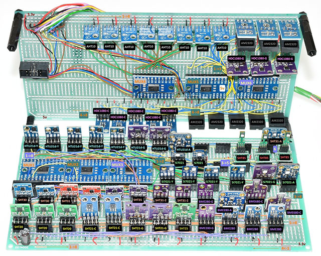
Once your project starts to grow it’s common to have multiple different sensors, from different vendors, measuring the same environmental parameter. Ideally, those sensors would produce the same readings but in practice there are significant offsets. Datasheets for the MS5837-02BA and MS5803-14BA that we will compare in this post claim an accuracy of (±0.5mbar) and (±2ºC) for the 2-bar while the 14-bar sensors are only rated to (±20mbar) and (±2ºC). Sensors from Measurement Specialties are directly code compatible so the units here were read with the same Over Sampling settings.

But this is only a starting point: manufacturers have very specific rules about things like the temperature ramps during reflow and it’s unlikely that cheap sensor modules get handled that carefully. Housing installation adds both physical stress and thermal mass which will induce shifts; as can the quality of your supply voltage. Signal conditioning and oversampling options usually improve accuracy, but there are notable exceptions like the BMP/E 280 which suffers from self-heating if you run it at the startup defaults.

Sensors like NTC thermistors are relatively easy to calibrate using physical constants. But finding that kind of high quality benchmark for barometric sensors is challenging if you don’t live near a government-run climate station. So we typically use a normalization process to bring a set of different sensors into close agreement with each other. This is a standard procedure for field scientists, but information on the procedures is hard to find because the word ‘normalization’ means different things in various industry settings. In Arduino maker forums it usually describes scaling the axes from a single accelerometer with (sensor – sensor.min )/( sensor.max – sensor.min ) rather than standardizing a group of different sensors.
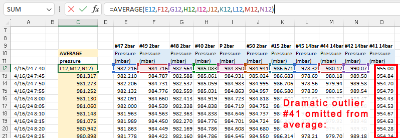
When calibrating to a good reference you generally assume that all the error is in your cheap DIY sensor and then do a linear regression by calculating a best fit line with the trusted data on they Y axis of a scatter plot. However, even in the absence of a established benchmark you can use the same procedure with a ‘synthetic’ reference created by drawing an average from your group of sensors:
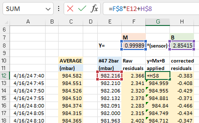
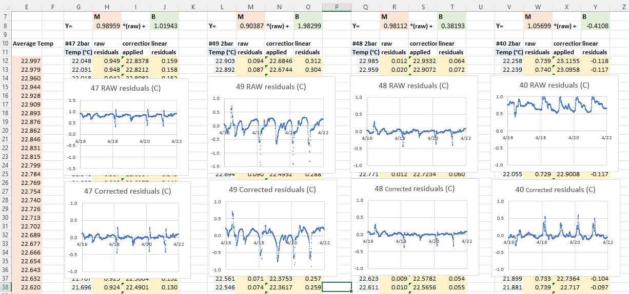
With that average you calculate y = Mx + B correction constants using Excel’s slope & intercept functions. Using these formulas lets you copy/paste equations from one data column to the next which dramatically speeds up the process when you are working through several sensors at a time. It also recalculates those constants dynamically when you add or delete information:
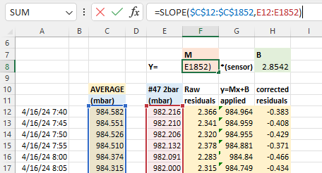
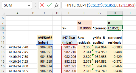
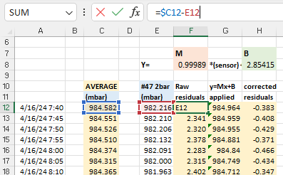
The next step is to calculate the difference (residuals) between the raw sensor data and the average: before and after these Y=Mx+B corrections have been applied to the original pressure readings. These differences between the group average and an individual sensor should be dramatically reduced by the Mx+b adjustments:
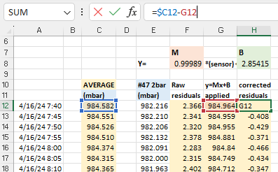
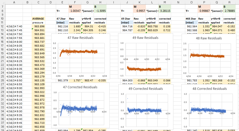
After you copy/paste these calculations to each sensor, create x/y scatter plots of the residuals so you can examine them side-by-side:

Now we can deal with the most important part of the entire process: Normalization with bad input data will produce even more misleading results. While the errors shown above are centered around zero, the patterns in these graphs indicate that we are not finished. In the ideal case, residuals should usually be soft fuzzy distributions with no observable patterns. But here we have a zigzag that is showing up for most of the sensors. This is an indication that one (or more) of the sensors included in the average has some kind of problem. Scrolling further along the columns identifies the offending sensors with nasty looking residual plots after the corrections have been applied:

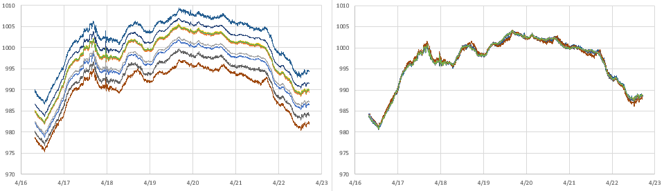
Sensor #41 (far right) was already rejected from the general average because of its enormous offset, but the high amplitude jagged residual plots indicate that the data from sensors #45 and #42 are also suspect. If we eliminate those two from the reference average the zigzag pattern disappears from the rest of the sensors in the set:
There’s more we could learn from the residual distributions, but here we’ve simply used them to prune our reference data, preventing bad sensor input from harming the the average we use for our normalization.
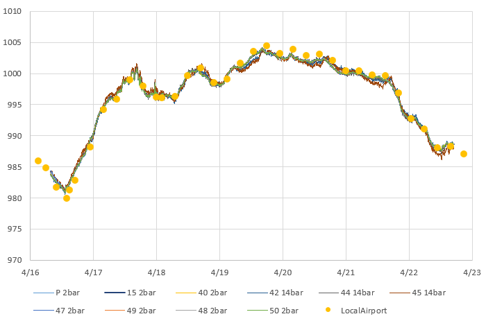
And what do the sensor plots look like after the magic sauce is applied?
It’s important to note that there is no guarantee that fitting your sensors to an average will do anything to improve accuracy. However, sensors purchased from different vendors, at different times, tend to have randomly distributed offsets. In that case normalization improves both precision and accuracy, but the only way to know if that has happened is to validate against some external reference like the weather station at your local airport. There are several good long term aggregators that harvest METAR data from these stations like this one at Iowa State, or you can get the most recent week of data by searching for your local airport code at weather.gov
METAR is a format for weather reporting that is predominately used for pilots and meteorologists and they report pressure adjusted to ‘Mean Sea Level’. So you will have to adjust your data to MSL (or reverse the correction on the airport data) before you can compare it to the pressure reported by your local sensors. For this you will also need to know the exact altitude of your sensors when the data was gathered to remove the height offset between your location and the airport stations.
Technically speaking, you could calibrate your pressure sensors directly to those official sources. However there are a lot of Beginner, Intermediate and Advanced details to take care of. Even then you still have to be close enough to know both locations are in the same weather system.
Here I’m just going to use the relatively crude adjustment equation:
Station Pressure = SLP – (elevation/9.2) and millibar = inchHg x 33.8639 to see if we are in the ballpark.
Like most pressure sensors an MS58xx also records temperature because it needs that for internal calculation. So we can repeat the entire process with the temperature readings from this sensor set:

These sensors were sitting pretty far back on a bookshelf that was partly enclosed, so some of them were quite sheltered while others were exposed to direct airflow. So I’m not bothered by the spikes or the corresponding blips in those residual plots. I’m confident that if I had run this test inside a thermally controlled environment (ie: a styrofoam cooler with a small hole in the top) the temperature residuals would have been well behaved.
One of the loggers in this set had a calibrated NTC thermistor onboard. While this sensor had significant lag because it was located inside the housing, we can still use it to check if the normalized temperatures benefit from the same random distribution of errors that were corrected so nicely by the pressure normalization:

Comments:
Normalization is a relatively low effort way to improve sets of sensors – and it’s vital if you are monitoring systems that are driven primarily by gradients rather than absolute values. This method generalizes to many other types of sensors although a simple y=Mx +B approach usually does not handle exponential sensors very well. As with calibration, the data set used for normalization should span the range of values you expect to gather with the sensors later on.
The method described here only corrects differences in Offset [with the B value] & Gain/Sensitivity [the M value] – more complex methods are needed to correct non-linearity problems. To have enough statistical power for accuracy improvement you want a batch of ten or more sensors and it’s a good idea to exclude data from the first 24 hours of operation so brand new sensors have time to settle. Offsets are influenced by several factors and some sensors need to ‘warm up’ before they can be read. The code driving your sensors during normalization should be identical to the code used to collect data in the field.
All sensor parameters drift so, just like calibration, normalization constants have a shelf life. This is usually about one year, but can be less than that if your sensors are deployed in harsh environments. Fortunately this kind of normalization is easy to redo in the field, and it’s a good way to spot sensors that need replacing. You could also consider airport/NOAA stations as stable references for drift determination.
References & Links:
Decoding Pressure @ Penn State
Environmental Mesonet @ Iowa State
Calibrating your Barometer: Part1, Part2 & Part3
How to Use Air Sensors: Air Sensor Guidebook
ISA Standard Atmosphere calculator
Starpath SLP calculator
SensorsONE Pressure Calculators
Mean Sea Level Pressure converter
I have to add a special mention here of the heroic effort by liutyi comparing different temp. & humidity sensors. While his goal was not normalization, the graphs clearly demonstrate how important that would be if you were comparing a group of sensors. Humidity sensors have always been a thorn in our side – both for lack of inter-unit consistency and because of their short lifespan in the field relative to other types of sensors. The more expensive Sensirons tend to last longer – especially if they are inside one of those protective shells made from sintered metal beads. KanderSmith also did an extensive comparison of humidity sensors with more detailed analysis of things like sensor response time.
You can use the map function to normalize range sensors where both the upper and lower bounds of the sensor varies. And you can use Binary Saturated Aqueous Solutions as standards.

Honestly as amazing as your hardware development is, these posts about calibration and validation are amazing, and ones I come back to again and again. I still need to write this stuff up, but theres still a books worth of work between where the average person (or student) is at and where you can take them. Thank you for this amazing resource… now if I can just digest it half as fast as you produce it.